
Friction define the coefficient of hydraulic resistance. Hydraulic friction coefficient
Ministry of Education and Science of the Russian Federation
National Research Nuclear University MEPhI
Balakovo Engineering and Technology
Determination of the coefficient of hydraulic friction of a straight pipe
Guidelines for performing laboratory work
disciplines: "Hydraulics", "Mechanics of fluid and gas", "Water supply and sanitation with the basics of hydraulics", "Hydrogasdynamics", "Hydraulics and hydropneumatic drive"
for students of the directions: "Heat power engineering and heat engineering", "Construction", "Design and technological support of machine-building industries", "Construction of unique buildings and structures", "Ground transport and technological means"
profile "Lifting and transport, construction, road facilities and equipment"
full-time, part-time and part-time reduced forms of education
Balakovo 2015
Objective:
1. Determine empirically the coefficient of hydraulic friction.
2. Determine the coefficient of hydraulic friction according to theoretical formulas and compare with the experimental value.
BASIC CONCEPTS
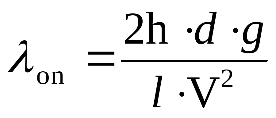
Loss of pressure due to friction along the length round pipes h l are determined by the Darcy formula:
where is the coefficient of hydraulic friction;
l is the length of the pipe on which the loss of pressure due to friction is determined;
d - pipe diameter;
V is the average fluid velocity;
g is the acceleration of gravity, equal to 981 cm / s 2.
Numerous experiments have established that the coefficient of hydraulic friction generally depends on the Reynolds number Re and the relative roughness of the pipe walls  :
:
 ,
(2)
,
(2)
where is the height of the roughness protrusions of the inner walls of the pipe.
The predominance of one or another factor depends on the fluid flow regime.
There are five zones hydraulic resistance.
1. Viscous resistance zone.
Movement laminar, Re< 2300. В этой зоне шероховатость стенок мало влияет на потери напора
 .
(3)
.
(3)
The theoretical formula for determining the coefficient of hydraulic friction for a round pipe follows from Poiseuille's law:
 .
(4)
.
(4)
2. Transition zone. At 2300< Re < 4000 имеет место переходная зона, в которой движение уже не ламинарное и еще не турбулентное, т. е. здесь режим неустойчивый. Инженерные расчеты в этой зоне выполняются очень редко.
3. Z o na hy d ra v l i ch e s and smooth d k i x p ub b. Turbulent movement 4000< Re < 10 5
. В этой зоне шероховатость стенок трубы
мало влияет на потери напора .
To determine the coefficient of hydraulic friction, there are many formulas, however, in this methodological instruction we present only one, the most applicable. For the zone of hydraulically smooth pipes, you can use the Blasius formula
 ;
(5)
;
(5)
4. Zone
t i v l e n i i. The movement is turbulent. Approximate boundaries of the zone
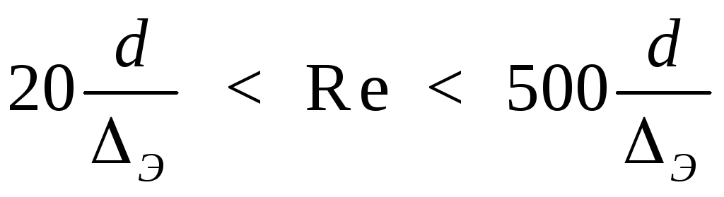 ,
,
where e is the value of the equivalent uniformly granular roughness.
Equivalent roughness is understood as such a uniformly-granular roughness, which in the region of quadratic resistance has the same resistance to fluid movement as a pipe with natural roughness. In this resistance zone, the coefficient of hydraulic friction depends on both factors 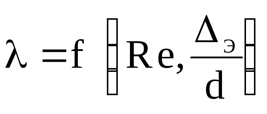 .
.
To determine the coefficient of hydraulic friction, you can use the formula A.D. Altshulya
 .
(6)
.
(6)
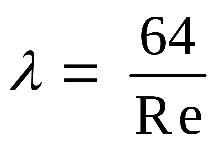
5. Zone of quadratic resistance.
The movement is turbulent. Lower zone limit  . In this zone, the main factor affecting the resistance is the roughness of the pipe walls.
  .
.
To determine the coefficient of hydraulic friction, you can use the following formula of B.L. Shifrinson
 .
(7)
.
(7)
EXPERIMENTAL TECHNIQUE
D e s c rip tio l
The diagram of the laboratory setup is shown in the figure. The laboratory setup consists of a pressure tank 1, a test pipe 2 with a diameter d. At the beginning and end of a pipe section with a length l piezometers 4 equipped with a measuring scale are connected through fittings and flexible hoses 3. The water flow in the test pipe is set using valve 5. Water is supplied to the pressure tank through pipe 6 using valve 7. To measure the water flow, a measuring tank 8 is used. Water is drained from the measuring tank through pipe 9 by opening valve 10. The water temperature is measured with a thermometer 11.
T e r o d i c o n s
Before carrying out the experiments, the pressure tank 1 is filled with water. In this case, valve 5 must be closed. Then the valve 5 opens and the flow rate Q is set in the interval 0< Q <= Q max. Обычно начинают с максимального расхода, соответствующего полному открытию вентиля 5. При проведении опытов необходимо поддерживать установившееся движение воды. Для этого при помощи вентиля 7 уровень воды в напорном баке 1
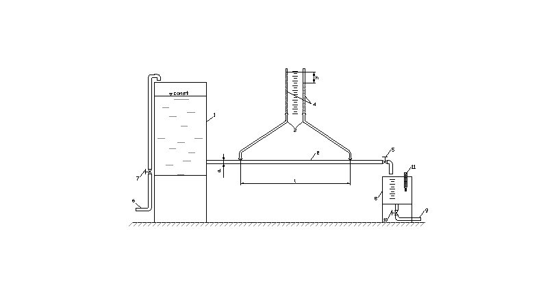 Scheme of the laboratory setup
kept constant. At a given water flow, the following measurements are made. With the help of piezometers 4, the difference in water levels in them is determined on a scale with an error of 0.5 mm. The line of sight must be perpendicular to the plane of the scale. At the same time, the water consumption is determined by the volumetric method using a measuring tank 8 and a stopwatch
The temperature of the liquid is necessary to determine the kinematic viscosity coefficient and is measured in the lower tank using a thermometer with an error ± 0.5 °C.
Water flow rates are set in such a way as to cover all resistance zones in the experiments.
SAFETY REQUIREMENTS
1. Before conducting experiments, it is necessary to study the instructions for the safety rules for working in the laboratory.
2. Study the description of the installation, prepare the necessary devices, clarify incomprehensible questions from the teacher. Start conducting experiments only with the permission of the teacher.
3. During the experiment, carefully handle glass and fragile instruments and equipment of the laboratory setup.
4. If there are difficulties in performing experiments, as well as breakage of instruments and equipment, it is necessary to stop the experiments and contact the teacher.
5. After completing the experiments, report to the teacher and hand over the instruments.
6. In case of injury, you must immediately stop the experiments and contact the teacher for medical help.
EXPERIMENTAL PROCEDURE
1. Preparation of the setup for the experiment.
1.1. Open valve 7 and fill pressure tank 1 with water up to the overflow level of the pressure tank. In this case, valve 5 must be closed.
1.3. The absence of water leaks at the junctions of flexible hoses 3 and through the valves is checked.
1.4. The length of the investigated pipe, the inner diameter, the roughness of the walls are determined.
1.5. Determine the dimensions of the measuring container.
2. Determination of coefficients of hydraulic friction empirically.
The maximum opening of the valve 5 sets the maximum water flow in the pipe.
With the help of the valve 7, a constant water level in the pressure tank 1 is achieved.
2.3. After reaching a steady state of motion on the scale determine the difference in water levels in the piezometers 4. The result is recorded in the table.
2.4. At the same time, the water flow rate is determined by the volumetric method and the water temperature is measured. When measuring the flow, the filling time of a given volume of the measuring vessel is determined.
2.6. After completion of all measurements in this experiment, valve 7 is closed first, then valve 5.
2.7. The table performs the necessary calculations to establish the resistance zone.
2.8. Valve 5 is opened less than the maximum, then with the help of valve 7 the water level in the pressure tank is maintained constant. Perform measurements similar to the first experiment.
2.9. When conducting experiments, they strive to cover all zones of resistance. The number of experiments must be at least four.
2.10. After completion of all experiments, valves 7 and 5 are closed, valve 10 is opened and checked for leaks in the valves, at the hose connections and in the hoses themselves.
PROCESSING THE EXPERIMENTAL RESULTS
The results of measurements and necessary calculations are entered in a table.
1. The cross-sectional area of the pipe is calculated S:
 (8)
(8)
where d - internal diameter of the pipe, cm.
2. Fluid flow is calculated Q , cm 3 /s.
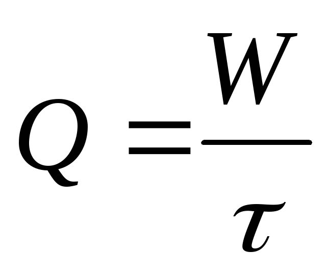 ,
(9)
,
(9)
where W- the volume of the measuring vessel, cm 3;
t is the filling time of the measuring tank, s.
3. The average fluid flow rate is calculated V:
 ,
,
 .
(10)
.
(10)
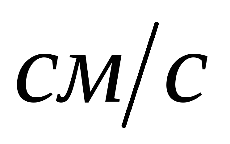
4. From the application, determine the kinematic coefficient of viscosity of water n cm 2 /s in accordance with the measured temperature °C.
5. Calculate the Reynolds number Re, corresponding to each experiment and set the zone of hydraulic resistance:
 (11)
(11)
6. Calculate the experimental value of the coefficient of hydraulic friction according to the formula
 .
(12)
.
(12)
7 Calculate the theoretical value of the coefficient of hydraulic friction according to the formula corresponding to the resistance zone.
8. Determine the discrepancy between the coefficients of hydraulic friction
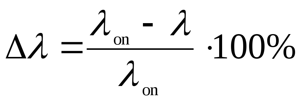 .
.
9. Draw conclusions about the correspondence between the theoretical and experimental coefficients of hydraulic friction and the nature of the change in the coefficient depending on the Reynolds number.
Determination of experimental error
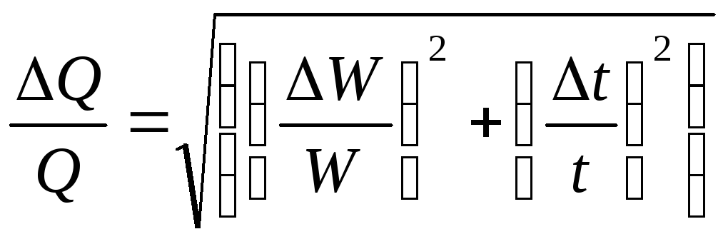
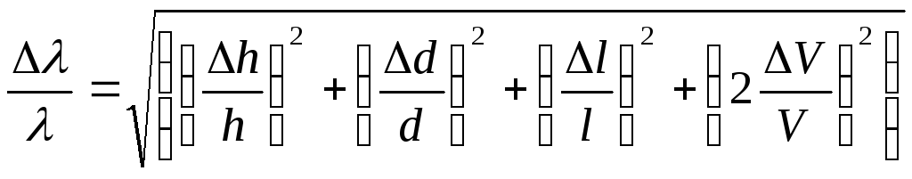
Random errors are neglected and only systematic errors are considered. The error in determining the area, flow rate, velocity and coefficient of hydraulic friction is found as an error in indirect measurements.
According to expressions (8) - (12), the relative error in determining the area, flow rate, speed and coefficient of hydraulic friction will be:
 ,
(13)
,
(13)
 ,
(14)
,
(14)
 ,
(15)
,
(15)
 ,
(16)
,
(16)
Through  the absolute measurement errors of individual quantities included in the expressions are indicated.
In this work, the filling time of the measuring tank, the water level in the piezometers and its temperature are experimentally measured.
The volume of the measuring vessel is determined with an error of DW = ± 10 cm 3, the time of its filling with an error of Dt = ± 0.2 s. The error of the kinematic coefficient of viscosity of water n is determined in accordance with the temperature measurement error. The water temperature is determined using a thermometer with an error of ± 0.5 °C. The inner diameter of the pipe is measured on a duplicate using a vernier caliper with an error of not more than 0.1 mm.
Errors according to formulas (13 - 16) are calculated for each resistance and all experiments. Next, an analysis of the results obtained is made, and ways to increase the accuracy of the experiments are outlined. In agreement with the teacher, each student of the link makes the calculation of one of the proposed measures to reduce the error. Based on the results of all calculations, a general conclusion is made about the possibility of increasing the accuracy of the experiments to the value specified by the teacher.
A report on the work of each student is drawn up in writing in a separate notebook and must contain:
1. The name of the laboratory work.
2. The formulation of the purpose of the work.
3. Some basic concepts and formulas.
4. Diagram and description of the laboratory setup.
5. Table with the results of the experiment.
6. Conclusions.
When handwritten, the installation diagram, tables are made in pencil using drawing instruments. It is desirable to run the report entirely on a computer.
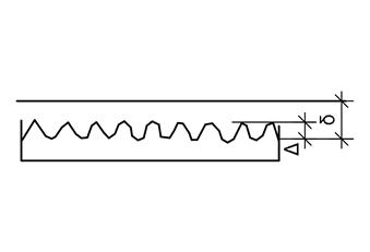
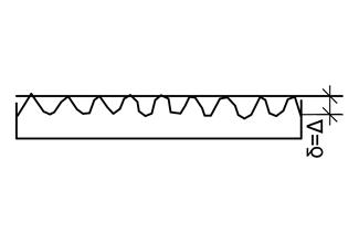
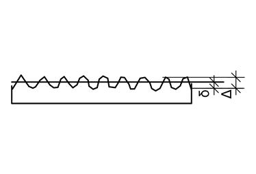
Depending on the ratio of the absolute height of the roughness projections Δ and the thickness of the viscous sublayer δ, the influence of viscous friction and inertial forces on shear stresses and energy losses in the flow manifests itself differently. The thickness of the viscous sublayer is determined
This value of δ should be compared with the height of the roughness ridges. Since the actual height of all protrusions is not the same, the concept is introduced equivalent roughness Δ equiv, i.e. such a uniform roughness, which, when calculated, gives the same value of the hydraulic friction coefficient λ with a given roughness. (Some values of the equivalent roughness are given in table. 111.1).
Table - Equivalent Roughness Values
Schematically, the following three areas of hydraulic resistance can be considered
1. Area of hydraulically smooth pipes: roughness protrusions are covered with a viscous sublayer (Δ equiv ‹ δ) and do not violate the integrity of the latter. The protrusions flow around without separations and vortex formations. In this case, the roughness does not affect the hydraulic resistance and the hydraulic coefficient of friction, which depends only on the Reynolds number. According to A. D. Altshul, this region exists at  <10.
<10.
For hydraulically smooth pipes, the Blasius formula is most widely used
Taking into account the dependence and the fact that, it is easy to verify that the pressure loss for hydraulically smooth pipes is proportional to the velocity to the power of 1.75.
k ch- coefficient of proportionality.
2. At > 500, there is a region of hydraulically rough pipes: the roughness protrusions go beyond the limits of the viscous sublayer (Δ eq > δ). The separated flow past the ledges reduces the friction resistance to the drag around bodies with a sharp change in configuration, which does not depend on the Reynolds number and is proportional to the velocity head of the flow and the size of the roughness ledges. It is these factors that are associated with the inertial resistances of the mixing particles of the liquid.
In the transition region of resistances, the hydraulic coefficient of friction can be determined by the formula of A. D. Altshul

3. At 10<экв в того же порядка, что и толщина вязкого подслоя δ. В этом случае на гидравлическое сопротивление влияют как число Рейнольдса, так и величина выступов шероховатости.
For hydraulically rough pipes, the formula turns into the Shifrinson formula
![]() .
.
Since in the latter case the coefficient of hydraulic friction does not depend on the speed of water movement, it follows from the formula that the head loss is proportional to the square of the speed
Hydraulic coefficient of friction (Darcy coefficient)
Based on the foregoing, taking into account the data of experimental studies, in general terms, the hydraulic coefficient of friction depends on the Reynolds number and the relative roughness of the pipe, i.e. ![]()
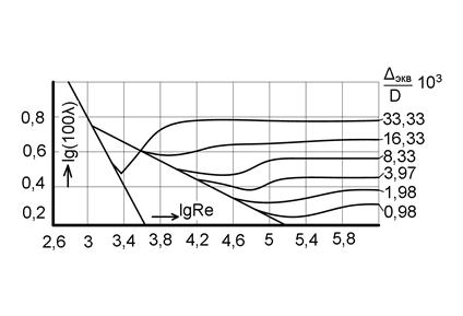
One of the most famous works in this area are the studies of I. Nikuradze, presented in the form of a graph in fig.
The graph shows that in the laminar regime λ depends only on the Reynolds number. At values Re = 2320-4000 in the zone of periodic regime change, λ grows rapidly. In the region of hydraulically smooth pipes, λ depends only on the Reynolds number, decreasing as the latter increases.
The transition region on the graph shows a family of curves for different relative roughnesses. In this region, the values of λ generally increase with an increase in the Reynolds number Re, but for small roughnesses, a decrease takes place in the initial section. In the field of hydraulically rough pipes, the coefficient λ is represented by a family of horizontal straight lines, different for different roughnesses.
It should be noted that the experiments of I. Nikuradze were carried out in pipes with artificial uniform roughness, glued to the pipe walls in the form of grains of sand of the same size. For practical purposes, the results of the experiments of K. Kolbrook, G. A. Murin, F. A. Shevelev and other scientists carried out for industrial pipes with natural uneven roughness are important. The generalized results of these studies are presented in the graph (Fig.), which, in contrast to the Nikuradze graph, shows that in the transition region, the values of λ are greater than in the quadratic region.
This important provision must be taken into account when calculating pipes operating in the transition region. It should also be noted that each pipe is not uniquely smooth or rough. Depending on the Reynolds number, the same pipe can work in the area of hydraulically smooth, rough pipes or in the transition area. In pipes with a relatively high roughness, upon transition to the turbulent regime, the viscous sublayer does not cover the roughness protrusions, and the area of hydraulically smooth pipes is absent. Depending on the characteristics of each area, there are various empirical formulas for determining the hydraulic coefficient of friction.
The Altshul formula is applicable to all resistance areas. At low Reynolds numbers, the value is much smaller than the value and can be neglected. In this case, the formula turns into the Blasius formula. For large Re numbers, the value can be neglected in comparison, and this formula turns into the Shifrinson formula.
For a number of special cases of fluid motion, there are separate empirical formulas for the hydraulic coefficient of friction. Asbestos-cement pipes usually work in the transition region of resistance. Non-new steel and cast iron pipes at water speeds V< 1,2 м/с также работают в переходной области сопротивления, а при V> 1.2 m/s - in the area of hydraulically rough pipes. F. A. Shevelev compiled tables for determining pressure losses in water pipes based on empirical formulas.
To calculate the movement of wastewater in drainage (sewer) pressure and non-pressure pipes the formula of N. F. Fedorov is applied

D = 4R - hydraulic diameter;
2 and a 2 - equivalent absolute roughness and dimensionless coefficient determined from the table;
Re - Reynolds number, in determining which the kinematic viscosity of wastewater is taken, depending on the amount of suspended particles in them, by 5-30% more than the viscosity of pure water.
Tab Odds? 2 and a 2 for N. F. Fedorov's formula
The values of the hydraulic coefficient of friction for wastewater are greater than when pure water moves in water pipes. N. F. Fedorov compiled on the basis of the table formula bandwidth and the rate of fluid flow in the drainage pipes.
Experiments, primarily G.A. Murin with technical pipelines showed that for a turbulent regime, λ changes not only with a change in the Re number, but the technical condition of the pipe also affects the value of λ. Murin examined 49 pipes made of various materials, used, with different diameters, at different speeds of fluid movement. The results of the experiments were obtained in the form of several curves (see Fig. 4.11).
Here, three regions of resistance are clearly distinguished in the turbulent regime. Line I corresponds to the area hydraulically smooth pipes , when the value of λ depends only on the number Re and does not depend on the material of the pipe. Mathematical data processing shows that for this area the dependence is regular
This dependence can be used in the range of Re numbers.
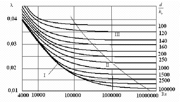
Rice. 4.11. Murin's chart
Region II on the chart is transitional range from hydraulically smooth to rough pipes. The value of λ depends both on the Re number and on . To determine λ in this region, the Altshul formula is best suited
which can be used for .
An analysis of the possible values of the coefficients of hydraulic friction for various conditions shows that pipelines for heat and gas supply and ventilation systems operate mainly in the transition region of resistance. Water lines most often belong to the area of rough pipes. How hydraulically smooth plastic, aluminum, brass pipes work.
The nature of the dependency curves  is determined by the nature of the fluid flow around the wall layer of roughness projections, which are always present on the pipe surface (Fig. 4.12).

Rice. 4.12. Fluid movement in hydraulically smooth and rough pipes
At low fluid velocities, the particles flow around the protrusions without the formation of vortices, which is explained by low inertial forces. Such a flow around the protrusions is typical for the region of hydraulically smooth pipes. With an increase in the speed of movement, the inertia forces of the fluid particles increase and separate vortices appear behind some roughness protrusions. The number of vortices and their magnitude increases with increasing fluid velocity. Such a flow pattern is characteristic of the transition region. With a further increase in the fluid flow rate, the vortices are located behind all the protrusions, their size does not change, which is typical for the area of hydraulically rough pipes. The size of the vortices depends, as we can see, on the size of the roughness protrusions, their shape, and the frequency of their distribution over the surface.
As an integral characteristic, the state of the inner surface of the pipe is used equivalent roughness , which is determined experimentally on the basis of hydraulic tests various pipelines and is given in reference books. Here are some values for pipes made of various materials:
Table 3-1
| Pipe material and condition | |
| From non-ferrous metals and glass |
Pipelines are widely used in metallurgical production for the transportation of liquids, gases, various pulps and mixtures. Existing water, gas, fuel oil, oxygen and other networks can be divided into two types: main pipelines, supplying this or that medium from the source to the consumer over long distances, and branched pipe networks that ensure the distribution of this medium directly to consumers.
The category of pipelines also includes various systems of flues and chimneys that serve to evacuate combustion products from the working space of metallurgical furnaces into chimney. The cross-sectional shape of such burs can be different, but they should not be distinguished from the class of pipes, since the formulas obtained for round pipes are valid for channels of any section, if we use the concept of hydraulic diameter.
All pipelines that do not have branches are called simple, even if they consist of sections of different diameters. Networks of pipes with branched and parallel sections are called complex pipelines.
In the general case, when calculating pipelines, one has to deal with the solution of three problems. In the first of them, for a given location of pipelines, length and diameter of pipes, it is required to determine the pressure difference required to pass a given flow rate of the medium Q. The second task is the reverse of the first. It needs to determine the cost Q if the pressure drop is known. The third task is to determine the diameter if all other parameters of the pipeline are known.
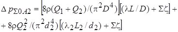
Simple pipelines . The method for calculating hydraulic resistance is based on the facts established earlier: the energy of a moving medium is spent to compensate for energy losses due to friction, local resistance and to overcome the effect of geometric pressure. In a simple pipeline, all loss sources are located successively, therefore, the total hydraulic resistance of such a pipeline can be represented by their algebraic sum, i.e.
When solving the first problem, all parameters of the pipeline are known; the flow rate of the medium is also given. In this regard, the speeds are also known, according to which the Reynolds numbers, friction coefficients, drag coefficients are calculated, if they depend on the speed, and according to the formula (8.41) the sum of all resistances is found, which determines the required pressure drop.
The second problem, as a rule, does not have a unique solution, since the coefficients and sometimes are functions of the Reynolds number, and it, in turn, is determined by the flow rate of the medium. Therefore, the method of successive approximations is usually used.
The third problem in the general case is also not uniquely solved, since in one equation of the type (8.41) all the diameters of the pipeline sections are unknown. If the segment is one and has length L, then a graphical solution is possible, the essence of which is as follows. They are set by a number of values of pipeline diameters , , …, ; for each solve the second problem and build dependency . Since the flow rate of the medium is given, then, using the constructed graph, you can find the desired diameter. For sections with a length and diameter d i The third problem can be solved by specifying additionally P- 1 ratio. Usually, in practice, such ratios are conditions that express the requirements for the minimum cost of the pipeline. This results in a typical optimization problem: to design a pipeline consisting of P sections of length in such a way that at a given flow rate, energy losses do not exceed, and the costs of its construction and operation are the least. Methods for solving such problems are beyond the scope of this course.
Complex pipelines . In a production environment, one has to deal with a wide variety of types of complex pipelines. However, almost all of them can be reduced to a combination in various proportions of three types of networks: parallel connection, ring pipeline and simple branched network.
Parallel connection (Fig. 8.13) is such a system when the pipeline at one point (for example, A) branches into P sections of length and diameter each, which are then at another point ( AT) merge into one channel again. In general, the diameters of the pipeline before branching and after merging can be different.

Rice. 8.13. Diagram of parallel connection of pipelines
A characteristic feature of the parallel connection of pipelines is that all its branches begin in the same section A, at pressure , and end in section B, at pressure . Therefore, the energy losses on each parallel branch are the same. Because of this, as well as under the assumption of a horizontal location of the pipeline, which allows us to neglect , we can write for the first branch:
 (8.42)
Denoting the expression in curly brackets through AT 1 , we get for the first branch and others:
![]()
![]()
![]() (8.43)
(8.43)
Since the left parts of all these ratios are the same, then all unknown costs can be expressed in terms of the consumption of the first branch, then
![]()
![]() (8.44)
(8.44)
Considering that the sum of expenses of each branch is equal to the total expense, i.e. , we get
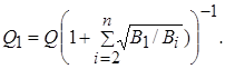 (8.45)
Having determined the expense, it is not difficult to find the expenses for other branches using formulas (8.44). Energy losses in this case are calculated according to equation (8.42). Since the costs are still unknown in the calculations, the method of iterations (successive approximations) is inevitable.
The coefficients have a certain physical meaning. Indeed, any channel can be replaced by a hole with area , which, when the same amount of gas flows, provides equivalent hydraulic resistance. The area of such a hole ![]() or taking into account the connection (8.43)
or taking into account the connection (8.43) ![]() . Thus, the coefficient determines the area of the hole, which is named equivalent. Using the concept of an equivalent hole, we can formulate a rule according to which in a system of parallel channels, costs are distributed in direct proportion to the areas of equivalent holes.
. Thus, the coefficient determines the area of the hole, which is named equivalent. Using the concept of an equivalent hole, we can formulate a rule according to which in a system of parallel channels, costs are distributed in direct proportion to the areas of equivalent holes.
Ring pipelines most typical for shaft furnaces with tuyere blast input (for example, blast furnaces). The main calculation task is to determine the pressure under conditions when the flow rates at the sampling points (nodal flow rates) , , ..., , the lengths of individual sections and the diameters of all pipes are given.
The most clear are the features of the method for calculating the ring pipeline, if we consider the simplest case of the presence of two nodal flow rates: (at point 1) and (at point 2) (Fig. 8.14).
Determining the pressure in the initial section of the pipeline is difficult because the energy losses are unknown, i.e., the path that each part of the total flow passes, and in what relation these parts are, is unknown. In this regard, the first step in the method for calculating the hydraulic resistance of an annular pipeline is to determine vanishing points, i.e. the point at which the parts of the general flow converge, initially branching at the point A.
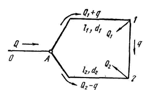
Rice. 8.14. Scheme of the ring pipeline
Suppose (see Fig. 8.14) that point 2 is such a point. In this case, on the section A-1 expense will be , on the site A -2 - Q 2 - and in section 1 - 2 - . Losses of energy from the main nodal point A up to the vanishing point, the "rings" are the same in both directions, i.e., or in expanded form
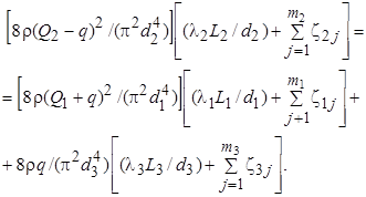 (8.46)
In this equation, the effect of geometric pressure is neglected, since pipelines of this kind are usually located horizontally. Since the second term on the right-hand side is positive, this relation is equivalent to the inequality
and especially
As mentioned earlier, the costs and parameters of pipelines are set, so the coefficient and is easily determined. Therefore, assessing the fairness of inequality is not difficult. If this inequality is true, then the vanishing point is point 2; otherwise, the vanishing point is point 1.
After the issue of the vanishing point is resolved, the desired initial pressure is determined by calculating the energy loss on a shorter path. In the context of our example ![]() . It should be borne in mind that in order to calculate this value, it is necessary to know the flow rate in section 1 - 2 q. The value is found from expression (8.46) or similar.
. It should be borne in mind that in order to calculate this value, it is necessary to know the flow rate in section 1 - 2 q. The value is found from expression (8.46) or similar.
In the conditions of metallurgical production, the number of lances of shaft furnaces (nodal costs) ranges from 4 to 24. Naturally, the calculation in this case becomes much more complicated. However, the methodology does not change fundamentally. And here the first step in the calculation is to establish the vanishing point.
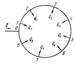 With 8 lances, this approach can be used to determine the vanishing point. Approximately as a vanishing point, a lance is chosen, located diametrically opposite to the main nodal point BUT(Fig. 8.15). Assuming that this is tuyere 4 and, taking into account that the distance between the tuyeres and the parameters of the sections and , are the same, except for the points closest to the point A, you can write:
Rice. 8.15. Scheme of blast supply to the shaft furnace
 (8.48)
Dropping , as before, leads to inequality (the right side must be greater than the left). It is generally desirable that the distribution of the blast over the tuyeres be uniform, i.e. ![]() Therefore, neglecting local resistances, we obtain
Therefore, neglecting local resistances, we obtain
In this inequality, it is calculated at the expense ![]() and etc.
and etc.
Let this inequality be satisfied. Does this mean that the lance is indeed a vanishing point? Apparently not, because equality does not have to be true - it is conjectural, and only proves that tuyere 3 is not a vanishing point. And what about tuyere 5? To do this, check if the inequality is true:
If this inequality holds together with the previous one, then tuyere 4 is indeed a vanishing point; otherwise, it will be lance 5. When this is also not obvious, as in this example, then lance 6 should be checked, and so on.
The calculation of the desired pressure is carried out along any path from point 0 to the vanishing point. In this case, it is found by an expression like (8.48). In practice, the inverse problem is more important and more common: to determine the distribution of blast over the tuyeres if the total flow rate , the pressure at the main point is 0, and the parameters of the pipeline and are given. Note that in this case it is required to jointly solve the problems of calculating the pipeline and the movement of bulk materials and gases in the furnace, since it is required to know the resistance to the outflow of blast from the tuyere to the bed for each tuyere.
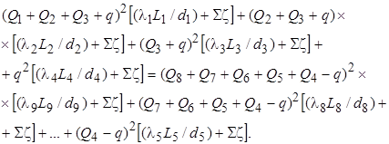
Simple branched network quite often found in metallurgical shops as an element of the design scheme of heating furnaces. These can be, for example, gas and air ducts that serve to supply gas and air to the furnace burner system, or, on the contrary, a system of flues and smoke channels that remove combustion products from several heating furnaces to one chimney.
The main tasks here can be considered the determination of end flow rates at a given pressure in the initial section or the determination of pressure at given end flow rates. Very often it is necessary to solve the third problem of finding the diameters of network sections when all other parameters are set.
 Let us consider the first problem as an example, and for simplicity we will assume that there are only two branches (Fig. 8.16). For definiteness, we will assume that we are talking about the supply of gas to the burners of the furnace.
Rice. 8.16. Diagram of a simple branched network
Since the gas is supplied to the same furnace, it is natural that the resistances on the branches will be the same. Then two relations can be written:
 (8.49)
 (8.50)
or, using the coefficients AT,
Subtracting the second equation from the first equation, we find
![]()
![]() (8.53)
(8.53)
those. costs in this case are distributed in direct proportion to the areas of equivalent holes. Substituting now equation (8.53) into (8.51), we obtain
 (8.54)
Note that here, as in determining costs, iteration over and is required.
It is easy to show that with branches the calculation scheme remains the same. It is only necessary to use relations (8.44) instead of equation (8.53), and replace (8.54) with the equation
 . (8.55)
A simple analysis of the above formulas shows that with the same branch diameters, the costs are distributed unevenly: the farther the nodal point is from the main point A, topics less consumption. Therefore, if it is necessary to ensure equality of the end flow rates, it is necessary to achieve the same areas of equivalent holes by appropriate selection of diameters, the degree of opening of the gate valves.
It follows from the foregoing that when determining the pressure in the case when the end flow rates are set, it is advisable to calculate the branch of the most distant point (from the main point A). The requirement to ensure the equality of the areas of equivalent holes at the same end costs remains in force here.
Chapter 9
The outflow of gases occurs during the operation of burners, nozzles, when gases are knocked out through holes in the walls of furnaces, and in many other cases.
The outflow of gases differs significantly from the outflow of liquids. When the liquid flows out, a simple process of realization of the stock of potential energy into the kinetic energy of the flow takes place; the temperature and density of the liquid do not change. During the outflow of gases, the potential energy reserve and part of the internal energy are simultaneously converted into kinetic energy, as a result of which the temperature and density of the gas can undergo significant changes.
However, if the outflow of gases occurs under the action of a very small pressure difference ( p£1.1 p env), then, as experience shows, the density of gases changes very slightly, so that this change in density can be neglected by setting r = r 0. Such a gas is conditionally called incompressible.