
Hydraulic calculation of the heat network calculation example. Hydraulic calculation of heat networks
To the task hydraulic calculation includes:
Determining the diameter of pipelines;
Determination of pressure drop (pressure);
Determination of pressures (heads) at various points in the network;
Coordination of all network points in static and dynamic modes in order to ensure acceptable pressures and required pressures in the network and subscriber systems.
According to the results of hydraulic calculation, the following tasks can be solved.
1. Determination of capital costs, consumption of metal (pipes) and the main scope of work for laying a heating network.
2. Determination of the characteristics of circulation and make-up pumps.
3. Determination of the operating conditions of the heating network and the choice of schemes for connecting subscribers.
4. The choice of automation for the heating network and subscribers.
5. Development of operating modes.
a. Schemes and configurations of thermal networks.
The scheme of the heat network is determined by the placement of heat sources in relation to the area of consumption, the nature of the heat load and the type of heat carrier.
The specific length of steam networks per unit of calculated heat load is small, since steam consumers - as a rule, industrial consumers - are located at a short distance from the heat source.
A more difficult task is the choice of the scheme of water heating networks due to the large length, a large number of subscribers. Water vehicles are less durable than steam ones due to greater corrosion, more sensitive to accidents due to the high density of water.
Fig.6.1. Single-line communication network of a two-pipe heat network
Water networks are divided into main and distribution networks. Through the main networks, the coolant is supplied from heat sources to the areas of consumption. Through distribution networks, water is supplied to the GTP and MTP and to subscribers. Subscribers rarely connect directly to backbone networks. Sectioning chambers with valves are installed at the distribution network connection points to the main ones. Sectional valves on main networks are usually installed after 2-3 km. Thanks to the installation of sectional valves, water losses during vehicle accidents are reduced. Distribution and main TS with a diameter of less than 700 mm are usually made dead-end. In case of accidents, for most of the country's territory, a break in the heat supply of buildings up to 24 hours is allowed. If a break in heat supply is unacceptable, it is necessary to provide for duplication or loopback of the TS.
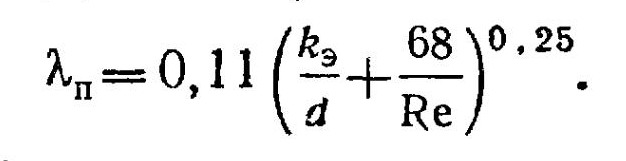
Fig.6.2. Ring heating network from three CHPPs Fig.6.3. Radial heating network
When supplying large cities with heat from several CHPs, it is advisable to provide for mutual blocking of CHPs by connecting their mains with blocking connections. In this case, a ring heating network with several power sources is obtained. Such a scheme has more high reliability, ensures the transfer of reserving water flows in case of an accident at any section of the network. With diameters of lines extending from the heat source of 700 mm or less, a radial scheme of the heat network is usually used with a gradual decrease in the diameter of the pipe as it moves away from the source and the connected load decreases. Such a network is the cheapest, but in the event of an accident, heat supply to subscribers is stopped.
b. Main calculated dependencies
Fig.6.1. Scheme of the movement of fluid in a pipe
The fluid velocity in pipelines is low, so the kinetic energy of the flow can be neglected. Expression H=p/r g is called the piezometric head, and the sum of the height Z and the piezometric head is called the total head.
H 0 \u003d Z + p/rg = Z + H.(6.1)
The pressure drop in the pipe is the sum of linear pressure losses and pressure losses due to local hydraulic resistances.
D p=D p l+d p m. (6.2)
In pipelines D p l = R l L, where R l is the specific pressure drop, i.e. pressure drop per unit length of the pipe, determined by the formula d "Arcy.
 . (6.3)
Coefficient hydraulic resistance l depends on the fluid flow regime and the absolute equivalent roughness of the pipe walls to e. You can take the following values in the calculations to e- in steam lines to e=0.2 mm; in water networks to e=0.5 mm; in condensate pipelines and hot water systems to e=1 mm.
For laminar fluid flow in a pipe ( Re < 2300)
In the transition region 2300< Re < 4000
 . (6.5)
At ![]()
![]() . (6.6)
. (6.6)
Usually in heating networks Re > Re pr, so (6.3) can be reduced to the form
 , where
 ![]() . (6.7)
. (6.7)
Pressure losses at local resistances are determined by the formula
 . (6.8)
Values of the coefficient of local hydraulic resistance x are given in reference books. In hydraulic calculations, pressure losses due to local resistances through the equivalent length can be taken into account.
Then where a=l equiv /l is the proportion of local pressure losses.
a. Hydraulic calculation procedure
Usually, in a hydraulic calculation, the flow rate of the coolant and the total pressure drop in the section are set. It is required to find the diameter of the pipeline. The calculation consists of two stages - preliminary and verification.
Estimation.
2. Specified by the proportion of local pressure drops a=0.3...0.6.
3. Estimate the specific pressure loss
 . If the pressure drop in the section is unknown, then they are given by the value R l < 20...30 Па/м.
4. Calculate the diameter of the pipeline from the conditions of operation in turbulent mode. For water heating networks, the density is assumed to be 975 kg/m 3 .
From (6.7) we find
 , (6.9)
where r- the average density of water in this area. According to the diameter value found, a pipe with the nearest inner diameter is selected according to GOST. When choosing a pipe, indicate either d and d, or d n and d.
2. Verification calculation.
For end sections, the driving mode should be checked. If it turns out that the movement mode is transient, then, if possible, it is necessary to reduce the diameter of the pipe. If this is not possible, then it is necessary to carry out the calculation according to the formulas of the transient mode.
1. Values are specified R l;
2. Types of local resistances and their equivalent lengths are specified. Gate valves are installed at the outlet and inlet of the collector, at the points of connection of distribution networks to the main ones, branches to the consumer and at consumers. If the branch length is less than 25 m, then it is allowed to install the valve only at the consumer. Sectional valves are installed after 1 - 3 km. In addition to gate valves, other local resistances are also possible - turns, changes in section, tees, merging and branching of the flow, etc.
To determine the number of temperature compensators, the lengths of the sections are divided by the allowable distance between the fixed supports. The result is rounded to the nearest whole number. If there are turns in the section, then they can be used for self-compensation of temperature elongations. In this case, the number of compensators is reduced by the number of turns.
5. The pressure loss in the area is determined. For closed systems Dp uch \u003d 2R l (l + l e).
For open systems, preliminary calculation is carried out according to the equivalent flow rate
![]()
In the verification calculation, the specific linear pressure losses are calculated separately for the supply and return pipelines for actual flow rates.
![]() ,
, ![]() .
.
At the end of the hydraulic calculation, a piezometric graph.
a. Piezometric graph of the heat network
On the piezometric graph, the relief of the terrain, the height of the attached buildings, and the pressure in the network are plotted on a scale. Using this graph, it is easy to determine the pressure and available pressure at any point in the network and subscriber systems.
The level 1 - 1 is taken as the horizontal reference plane for the pressures. Line P1 - P4 - the graph of the pressures of the supply line. Line O1 - O4 - graph of the pressure of the return line. H o1 - full pressure on the return collector of the source; Hsn - pressure of the network pump; Нst is the total head of the make-up pump, or the total static head in the heating network; Hk - total pressure in t.K on the discharge pipe of the network pump; DHt - pressure loss in the heat-preparation plant; Np1 - full pressure on the supply manifold, Np1 \u003d Hk - DHt. The available pressure of network water on the collector of the CHPP is H1=Np1-No1. The pressure at any point in the network i is denoted as Npi, Hoi - total heads in the forward and return pipelines. If the geodetic height at point i is Zi, then the piezometric head at this point is Hpi - Zi, Hoi - Zi in the straight line and return pipelines, respectively. The available pressure at point i is the difference between the piezometric pressures in the forward and return pipelines - Нпi - Hoi. The available pressure in the TS at the subscriber's connection point D is H4 = Hp4 - No4.
Fig.6.2. Scheme (a) and piezometric graph (b) of a two-pipe heating network
There is a pressure loss in the supply line in section 1 - 4. There is a pressure loss in the return line in section 1 - 4 ![]() . During the operation of the network pump, the pressure Hst of the feed pump is regulated by the pressure regulator up to No1. When the network pump stops, a static head Hst is established in the network, developed by the make-up pump. In the hydraulic calculation of the steam pipeline, the profile of the steam pipeline can be ignored due to the low steam density. Pressure loss at subscribers, for example
. During the operation of the network pump, the pressure Hst of the feed pump is regulated by the pressure regulator up to No1. When the network pump stops, a static head Hst is established in the network, developed by the make-up pump. In the hydraulic calculation of the steam pipeline, the profile of the steam pipeline can be ignored due to the low steam density. Pressure loss at subscribers, for example ![]() depends on the connection scheme of the subscriber. With elevator mixing D H e = 10 ... 15 m, with elevatorless input - D nb e = 2 ... 5 m, in the presence of surface heaters D H n=5…10 m, with pump mixing D H ns= 2…4 m.
depends on the connection scheme of the subscriber. With elevator mixing D H e = 10 ... 15 m, with elevatorless input - D nb e = 2 ... 5 m, in the presence of surface heaters D H n=5…10 m, with pump mixing D H ns= 2…4 m.
Requirements for the pressure regime in the heating network:
b. at any point in the system, the pressure must not exceed the maximum allowable value. Pipelines of the heat supply system are designed for 16 atm, pipelines of local systems - for pressure of 6-7 atm;
c. in order to avoid air leaks at any point in the system, the pressure must be at least 1.5 atm. In addition, this condition is necessary to prevent pump cavitation;
d. at any point in the system, the pressure must not be less than the saturation pressure at a given temperature in order to prevent water from boiling;
6.5. Features of the hydraulic calculation of steam pipelines.
The diameter of the steam line is calculated based on either the allowable pressure loss or the allowable steam velocity. The steam density in the calculated section is preliminarily set.
Calculation of admissible pressure losses.
Appreciate  , a= 0.3...0.6. According to (6.9), the pipe diameter is calculated.
Set by the speed of steam in the pipe. From the equation for steam flow - G=wrF find the pipe diameter.
According to GOST, a pipe with the nearest inner diameter is selected. Specific linear losses and types of local resistances are specified, equivalent lengths are calculated. The pressure at the end of the pipeline is determined. Heat losses are calculated in the design area according to normalized heat losses.
Qpot=q l l, where q l- heat loss per unit length for a given difference in steam temperatures and environment taking into account heat losses on supports, valves, etc. If a q l determined without taking into account heat losses on supports, valves, etc., then
Qpot \u003d q l (tav - to) (1 + b), where tav- average steam temperature in the area, to- ambient temperature, depending on the laying method. For ground laying to = tno, for underground channelless laying to = tgr(soil temperature at the laying depth), when laying in through and semi-through channels to= 40 ... 50 0 С. When laying in impassable channels to= 5 0 C. Based on the found heat losses, the change in the enthalpy of steam in the section and the value of the enthalpy of steam at the end of the section are determined.
Diuch=Qpot/D, ik=in - Diuch.
Based on the found values of steam pressure and enthalpy at the beginning and end of the section, a new value of the average steam density is determined rav = (rн + rk)/2. If the new density value differs from the previously specified one by more than 3%, then the verification calculation is repeated with clarification at the same time and Rl.
a. Features of the calculation of condensate pipelines
When calculating the condensate pipeline, it is necessary to take into account the possible vaporization when the pressure drops below the saturation pressure (secondary steam), steam condensation due to heat losses and passing steam after the steam traps. The amount of passing steam is determined by the characteristics of the steam trap. The amount of condensed steam is determined by the heat loss and the heat of vaporization. The amount of secondary steam is determined by the average parameters in the design area.
If the condensate is close to saturation, then the calculation should be carried out as for a steam pipeline. When transporting supercooled condensate, the calculation is carried out in the same way as for water networks.
b. Network pressure mode and choice of subscriber input scheme.
1. For normal operation of heat consumers, the pressure in the return line must be sufficient to fill the system, Ho > DHms.
2. The pressure in the return line must be below the permissible value, po > pperm.
3. The actual available pressure at the subscriber's input must not be less than the calculated one, DHab DHcalc.
4. The pressure in the supply line must be sufficient to fill the local system, Hp - DHab > Hms.
5. In static mode, i.e. when turning off the circulation pumps, there must be no emptying of the local system.
6. Static pressure must not exceed the allowable.
Static pressure is the pressure that is set after the circulation pumps are switched off. The level of static pressure (pressure) must be indicated on the piezometric graph. The value of this pressure (pressure) is set based on the limitation of the pressure value for heating appliances and must not exceed 6 ati (60 m). With a calm terrain, the level of static pressure can be the same for all consumers. With large fluctuations in the terrain, there may be two, but not more than three static levels.
Fig.6.3. Graph of static pressures of the heating system
Figure 6.3 shows a graph of static pressure and a diagram of the heat supply system. The height of buildings A, B and C is the same and equal to 35 m. If you draw a line of static pressure 5 meters above building C, then buildings B and A will be in a pressure zone of 60 and 80 m. The following solutions are possible.
7. Heating installations of buildings A are connected according to an independent scheme, and in buildings B and C - according to a dependent one. In this case, a common static zone is established for all buildings. Water-water heaters will be under pressure of 80 m, which is acceptable in terms of strength. Line of static pressure - S - S.
8. Heating installations of building C are connected according to an independent scheme. In this case, the total static head can be selected according to the strength conditions of the installations of buildings A and B - 60 m. This level is indicated by the line M - M.
9. The heating installations of all buildings are connected according to a dependent scheme, but the heat supply zone is divided into two parts - one M-M level for buildings A and B, the other on S-S level for building C. To do this, between buildings B and C, a check valve 7 is installed on the direct line and a make-up pump of the upper zone 8 and a pressure regulator 10 on the return line. The specified static head in zone C is maintained by the booster pump of the upper zone 8 and the boost controller 9. The preset static head in the lower zone is maintained by pump 2 and the controller 6.
In the hydrodynamic mode of the network, the above requirements must also be observed at any point in the network at any water temperature.
Fig.6.4. Plotting a graph of hydrodynamic pressures of a heat supply system
10. Construction of lines of maximum and minimum piezometric heads.
The lines of permissible pressures follow the terrain, because it is assumed that pipelines are laid in accordance with the relief. Reading - from the axis of the pipe. If the equipment has significant dimensions in height, then the minimum pressure is counted from the upper point, and the maximum - from the lower one.
1.1. The Pmax line is the line of the maximum allowable pressure in the supply line.
For peak hot water boilers, the maximum allowable head is measured from the lower point of the boiler (it is assumed that it is at ground level), and the minimum allowable head is measured from the upper collector of the boiler. Permissible pressure for steel boilers 2.5 MPa. Taking into account the losses, Hmax=220 m is assumed at the outlet of the boiler. The maximum allowable pressure in the supply line is limited by the strength of the pipeline (рmax=1.6 MPa). Therefore, at the entrance to the supply line, Hmax = 160 m.
a. The Omax line is the line of the maximum allowable pressure in the return line.
According to the strength condition of water-to-water heaters, the maximum pressure should not exceed 1.2 MPa. Therefore, the maximum head value is 140 m. The head value for heating installations cannot exceed 60 m.
The minimum allowable piezometric head is determined by the boiling temperature, which is 30 0 C higher than the calculated temperature at the outlet of the boiler.
b. Pmin line - the line of the minimum allowable head in a straight line
The minimum allowable pressure at the outlet of the boiler is determined from the condition of non-boiling at the upper point - for a temperature of 180 0 C. It is set to 107 m. From the condition of non-boiling water at a temperature of 150 0 C, the minimum head should be 40 m.
1.4. The Omin line is the line of the minimum allowable head in the return line. From the condition of inadmissibility of air leaks and cavitation of pumps, a minimum head of 5 m was adopted.
The actual pressure lines in the forward and reverse lines under no circumstances can go beyond the lines of maximum and minimum pressures.
The piezometric graph gives a complete picture of the acting heads in static and hydrodynamic modes. In accordance with this information, one or another method of connecting subscribers is selected.
Fig.6.5. Piezometric graph
Building 1. The available pressure is more than 15 m, piezometric - less than 60 m. It is possible to connect the heating installation according to a dependent scheme with an elevator assembly.
Building 2. In this case, you can also apply dependent schema, but because the pressure in the return line is less than the height of the building in the connection point, it is necessary to install a pressure regulator "to yourself". The differential pressure across the regulator must be greater than the difference between the installation height and the piezometric head in the return line.
Building 3. The static head in this place is more than 60 m. It is best to use an independent scheme.
Building 4. The available pressure in this place is less than 10 m. Therefore, the elevator will not work. You need to install a pump. Its pressure must be equal to the pressure loss in the system.
Building 5. It is necessary to use an independent scheme - the static head in this place is more than 60 m.
6.8. Hydraulic mode of heating networks
The pressure loss in the network is proportional to the square of the flow
Using the formula for calculating pressure losses, we find S.
![]() .
.
The head loss in the network is defined as , where ![]() .
.
When determining the resistance of the entire network, the following rules apply.
1. When the network elements are connected in series, their resistances are summed up S.
S S=S si.
11. When the network elements are connected in parallel, their conductivities are summed up.
 .
. ![]() .
.
One of the tasks of the hydraulic calculation of the TS is to determine the water consumption for each subscriber and in the network as a whole. Usually known: network diagram, resistance of sections and subscribers, available pressure on the collector of a CHP or boiler house.
![]()
Rice. 6.6. Heat network diagram
Denote S I- S V - resistance sections of the highway; S 1 – S 5 - resistance of subscribers together with branches; V- total water consumption in the network, m 3 / s; Vm– water consumption through a subscriber installation m; SI-5– resistance of network elements from section I to branch 5; SI-5=S I+ S 1-5, where S 1-5 - the total resistance of subscribers 1-5 with the corresponding branches.
The water flow through installation 1 is found from the equation
![]() , hence
, hence  .
.
For indoor installation 2
![]() . We find the difference in costs from the equation
. We find the difference in costs from the equation
![]() , where
, where ![]() . From here
. From here
 .
.
For setting 3 we get

Resistance of the heating network with all branches from subscriber 3 to the last subscriber 5 inclusive; ![]() , - resistance of section III of the highway.
, - resistance of section III of the highway.
For some m-th consumer from n the relative water flow is found by the formula
 . Using this formula, you can find the water flow through any subscriber installation, if the total flow in the network and the resistance of the network sections are known.
12. The relative water flow through the subscriber installation depends on the resistance of the network and subscriber installations and does not depend on the absolute value of the water flow.
13. If connected to the network n subscribers, then the ratio of water consumption through installations d and m, where d < m, depends only on the resistance of the system, starting from the node d to the end of the network, and does not depend on the resistance of the network to the node d.
If resistance changes at any section of the network, then all subscribers located between this section and the end point of the network will change the water flow proportionally. In this part of the network, it is sufficient to determine the degree of change in the consumption of only one subscriber. When the resistance of any element of the network changes, the flow rate will change both in the network and for all consumers, which leads to misalignment. Misadjustments in the network are corresponding and proportional. With a corresponding misadjustment, the sign of the change in costs coincides. With proportional misalignment, the degree of change in costs coincides.
Rice. 6.7. Change in network pressure when one of the consumers is turned off
If subscriber X is disconnected from the heating network, then the total resistance of the network will increase (parallel connection). The water flow in the network will decrease, the pressure loss between the station and the subscriber X will decrease. Therefore, the pressure graph (dotted line) will go more smoothly. The available pressure at point X will increase, so the flow in the network from subscriber X to the end point of the network will increase. For all subscribers from point X to the end point, the degree of change in flow will be the same - proportional misalignment.
![]()
For subscribers between the station and point X, the degree of change in consumption will be different. The minimum degree of change in consumption will be at the first subscriber directly at the station - f=1. As you move away from the station f > 1 and increases. If the available pressure at the station changes, then the total water consumption in the network, as well as the water consumption of all subscribers, will change in proportion to the square root of the available pressure at the station.
6.9. network resistance.
Total network conductivity
 , hence
 .
.
Similarly
 and
and
 . The calculation of the network resistance is carried out from the most remote subscriber.
a. Inclusion of pumping substations.
Pumping substations can be installed on the supply, return pipelines,
and also on the jumper between them. The construction of substations is caused by unfavorable terrain, long transmission distance, the need to increase the bandwidth, etc.
a). Installation of a pump on the supply or return lines.
Fig.6.8. Installing a pump in a supply or series line (serial operation)
When installing a pumping substation (NP) on the supply or return lines, the water consumption for consumers located between the station and the NP decreases, and for consumers after the NP they increase. In the calculations, the pump is taken into account as a certain hydraulic resistance. The calculation of the hydraulic regime of the network with NP is carried out by the method of successive approximations.
Set by the negative value of the hydraulic resistance of the pump
Calculate resistance in the network, water consumption in the network and at consumers
The water flow rate and the pump pressure and its resistance are specified by (*).
Fig.6.10. Total characteristics of series and parallel connected pumps
When the pumps are connected in parallel, the total characteristic is obtained by summing the abscissas of the characteristics. When the pumps are connected in series, the total characteristic is obtained by summing the ordinates of the characteristics. The degree of change in supply when the pumps are connected in parallel depends on the type of network characteristic. The lower the resistance of the network, the more efficient the parallel connection and vice versa.
Fig.6.11. Parallel connection of pumps
When the pumps are connected in series, the total water supply is always greater than the water supply by each of the pumps individually. The greater the resistance of the network, the more efficient the series connection of the pumps.
b). Installation of the pump on the jumper between the supply and return lines.
When installing the pump on the jumper temperature regime before and after NP is not the same.
To build the total characteristic of two pumps, the characteristic of pump A is first transferred to node 2, where pump B is installed (see Fig. 6.12). On the given characteristic of the pump A2 - 2, the heads at any flow rate are equal to the difference between the actual head of this pump and the head loss in the network C for the same flow rate.
![]() . After bringing the characteristics of pumps A and B to the same common node, they are added according to the rule of addition of pumps operating in parallel. When one pump B is operating, the pressure in node 2 is equal to , water flow. When the second pump A is connected, the pressure in node 2 increases to , and the total water flow increases to V>. However, the direct supply of pump B is reduced to .
. After bringing the characteristics of pumps A and B to the same common node, they are added according to the rule of addition of pumps operating in parallel. When one pump B is operating, the pressure in node 2 is equal to , water flow. When the second pump A is connected, the pressure in node 2 increases to , and the total water flow increases to V>. However, the direct supply of pump B is reduced to .
Fig.6.12. Building a hydraulic characteristic of a system with two pumps in different nodes
a. Network operation with two power supplies
If the vehicle is powered by several heat sources, then in the main lines there are points of meeting of water flows from different sources. The position of these points depends on the resistance of the vehicle, the distribution of the load along the main, and the available pressures on the collectors of the CHP. The total water consumption in such networks is usually given.
Fig.6.13. Scheme of a vehicle powered by two sources
The watershed point is found as follows. They are set by arbitrary values of water flow in sections of the highway based on the 1st Kirchhoff law. The head residuals are determined on the basis of the 2nd Kirchhoff law. If, with a pre-selected flow distribution, the watershed is selected in t.K, then the second Kirchhoff equation will be written in the form - pressure drop at the consumer m + 1 when powered from station B. or .
2. According to the equation (*), the second is calculated.
3. Calculate the resistance of the network and the flow rates of water supplied from stations A and B.
4. Calculate the consumption of water at the consumer - and.
5. The condition is checked
![]() ,
, ![]() .
.
a. Ring network.
The ring network can be considered as a network with two power supplies with equal heads of network pumps. The position of the watershed point in the supply and return lines is the same if the resistances of the supply and return lines are the same and there are no booster pumps. Otherwise, the positions of the watershed point in the supply and return lines must be determined separately. The installation of a booster pump leads to a displacement of the watershed point only in the line on which it is installed.
Fig.6.15. Diagram of pressure in the ring network
In this case ON = HB.
b. Switching on pumping substations in a network with two power supplies
To stabilize the pressure regime in the presence of a booster pump at one of the stations, the pressure on the inlet manifold is maintained constant. This station is called fixed, the other stations are called free. When a booster pump is installed, the pressure in the inlet manifold of a free station changes by .
a. Hydraulic mode of open heat supply systems
The main feature of the hydraulic mode of open heat supply systems is that in the presence of water intake, the water flow in the return line is less than in the supply line. In practice, this difference is equal to the water intake.
Fig.6.18. Piezometric plot of an open system
The piezometric curve of the supply line remains constant for any water withdrawal from the return line, since the flow in the supply line is kept constant by means of flow regulators on the subscriber inlets. With an increase in water intake, the flow in the return line decreases and the piezometric curve of the return line becomes flatter. When the draw-off is equal to the flow in the flow, the flow in the return is zero and the piezometric curve of the return line becomes horizontal. With the same diameters of the direct and return lines and the absence of water intake, the head graphs in the direct and return lines are symmetrical. In the absence of water intake for hot water supply, the water consumption is equal to the estimated heating consumption - V.
From equation (***) one can find f.

1. When DHW is drawn from the supply line, the flow through the heating system drops. When parsing from the reverse line, it grows. At b=0.4 water flow through the heating system is equal to the calculated one.
2. The degree of change in water flow through the heating system -
3. The degree of change in water flow through the heating system is the greater, the lower the resistance of the system.
An increase in the DHW drawdown can lead to a situation where all the water after the heating system will go to the DHW drawdown. In this case, the water flow in the return pipeline will be equal to zero.
From (***): ![]() , where (****)
, where (****)
Page 1
The hydraulic calculation is essential element design of thermal networks.
The task of hydraulic calculation includes:
1. Determination of pipeline diameters,
2. Determination of the pressure drop in the network,
3. Establishing the magnitude of pressure (pressure) at various points in the network,
4. Coordination of pressures at various points of the system in static and dynamic modes of its operation,
5. Establishment of the necessary characteristics of circulation, booster and make-up pumps, their number and location.
6. Determination of methods for connecting subscriber inputs to the heating network.
7. Selection of schemes and devices for automatic control.
8. Identification of rational modes of operation.
Hydraulic calculation is carried out in the following order:
1) in the graphic part of the project, a general plan of the city district is drawn on a scale of 1: 10000, in accordance with the task, the location of the heat source (HS) is applied;
2) show the scheme of the heat network from IT to each microdistrict;
3) for the hydraulic calculation of the heat network on the pipeline route, the main design line is selected, as a rule, from the heat source to the most remote heat unit;
4) on the calculation scheme indicate the numbers of sections, their lengths, determined according to the general plan, taking into account the accepted scale, and the estimated water flow;
5) on the basis of coolant flow rates and, focusing on a specific pressure loss of up to 80 Pa / m, designate the diameters of pipelines in sections of the main;
6) according to the tables, determine the specific pressure loss and coolant velocity (preliminary hydraulic calculation);
7) calculate the branches according to the available pressure drop; in this case, the specific pressure loss should not exceed 300 Pa / m, the coolant velocity - 3.5 m / s;
8) draw a diagram of pipelines, arrange shut-off valves, fixed supports, compensators and other equipment; distances between fixed supports for sections of different diameters are determined based on the data in table 2;
9) based on local resistances, determine the equivalent lengths for each section and calculate the reduced length using the formula:
10) calculate the pressure loss in the sections from the expression
![]() ,
,
Where α is a coefficient that takes into account the proportion of pressure losses at local resistances;
∆ptr is the pressure drop due to friction in the section of the heating network.
The final hydraulic calculation differs from the preliminary one in that the pressure drop due to local resistances is taken into account more accurately, i.e. after the arrangement of compensators and shut-off fittings. Gland expansion joints are used for d ≤ 250 mm, for smaller diameters - U-shaped expansion joints.
Hydraulic calculation is performed for the supply pipeline; the diameter of the return pipeline and the pressure drop in it are taken to be the same as in the supply pipeline (clause 8.5).
According to clause 8.6, the smallest internal diameter of pipes should be taken in heating networks at least 32 mm, and for hot water circulation pipelines - at least 25 mm.
The preliminary hydraulic calculation starts from the last section from the heat source and is summarized in Table 1.
Table 6 - Preliminary hydraulic calculation
|
plot number |
lpr=lx (1+α), m |
∆Р=Rхlpr, Pa | |||||||
|
HIGHWAY |
|||||||||
|
SETTLEMENT BRANCH |
|||||||||
|
∑∆Rotv = | |||||||||
Cons_6.doc
6. HYDRAULIC CALCULATION OF THERMAL NETWORKS
The task of hydraulic calculation includes:Determining the diameter of pipelines;
Determination of pressure drop (pressure);
Determination of pressures (heads) at various points in the network;
Coordination of all network points in static and dynamic modes in order to ensure acceptable pressures and required pressures in the network and subscriber systems. According to the results of hydraulic calculation, the following tasks can be solved.
Determination of capital costs, consumption of metal (pipes) and the main scope of work for laying a heating network.
Determination of the characteristics of circulation and make-up pumps.
Determination of the operating conditions of the heating network and the choice of schemes for connecting subscribers.
The choice of automation for the heating network and subscribers.
Development of operating modes.
6.1. Schemes and configurations of heat networks
The scheme of the heat network (TS) is determined by the placement of heat sources in relation to the area of consumption, the nature of the heat load and the type of heat carrier. The specific length of steam networks per unit of calculated heat load is small, since steam consumers - as a rule, industrial consumers - are located at a short distance from the heat source.
A more difficult task is the choice of the scheme of water heating networks due to the large length, a large number of subscribers. Water vehicles are less durable than steam ones due to greater corrosion, more sensitive to accidents due to the high density of water.
Fig.6.1. Single-line communication network of a two-pipe heat network
Water networks are divided into main and distribution networks. Through the main networks, the coolant is supplied from heat sources to the areas of consumption. Through distribution networks, water is supplied to group and local heating points (GTP and MTP) and to subscribers. Subscribers rarely connect directly to backbone networks. Sectioning chambers with valves are installed at the distribution network connection points to the main ones. Sectional valves on main networks are usually installed after 2 ... 3 km. Thanks to the installation of sectional valves, water losses during vehicle accidents are reduced. Distribution and main TS with a diameter of less than 700 mm are usually made dead-end. In case of accidents, for most of the country's territory, a break in the heat supply of buildings up to 24 hours is allowed. If a break in heat supply is unacceptable, it is necessary to provide for duplication or loopback of the TS.
When supplying large cities with heat from several CHPs, it is advisable to provide for mutual blocking of CHPs by connecting their mains with blocking connections. In this case, a ring heating network with several power sources is obtained. Such a scheme has a higher reliability, provides the transfer of reserving water flows in case of an accident in any section of the network. When the diameters of the mains extending from the heat source are 700 mm or less, a radial scheme of the heat network is usually used with a gradual decrease in the diameter of the pipe as it moves away from the source and the connected load decreases. Such a network is the cheapest, but in the event of an accident, heat supply to subscribers is stopped. 
Fig.6.2. Ring heating network from three CHPPs Fig.6.3. Radial heating network
^
6.2. Main calculated dependencies
 | The one-dimensional steady motion of a fluid in a pipe (see Fig. 6.4) is described by the Bernoulli equation
Z 1 , Z 2 - geometric height of the pipe axis in sections 1 and 2; w 1 and w 2 – fluid motion velocities in sections 1 and 2; p 1 and p 2 – fluid pressure on the pipe axis in sections 1 and 2; D p- pressure drop in segment 1-2; g- acceleration of free |
 , where
Fig.6.4. Scheme of the movement of fluid in a pipe
fall. Bernoulli's equation can be written for heads by dividing both parts by g.The fluid velocity in pipelines is low, so the kinetic energy of the flow can be neglected. Expression H=p/r g is called the piezometric head, and the sum of the height Z and the piezometric head is called the total head.
H 0 =Zp/rg = ZH.(6.1)
The pressure drop in the pipe is the sum of linear pressure losses and pressure losses due to local hydraulic resistances.
D p=D p l D p m. (6.2)
In pipelines D p l = R l L, where R l is the specific pressure drop, i.e. pressure drop per unit length of the pipe, determined by the formula d "Arcy.
 . (6.3)
The coefficient of hydraulic resistance l depends on the fluid flow regime and the absolute equivalent roughness of the pipe walls to e. You can take the following values in the calculations to uh - in steam lines to e = 0.2 mm; in water networks to e =0.5 mm; in condensate pipelines and hot water systems to e \u003d 1 mm.
For laminar fluid flow in a pipe ( Re < 2300)
 . (6.4)
In the transition region 2300< Re < 4000
 . (6.5)
At 
 . (6.6)
Usually in heating networks Re > Re pr, therefore (6.3) can be reduced to the form
 , where
  . (6.7)
Pressure losses at local resistances are determined by the formula
 . (6.8)
Values of the coefficient of local hydraulic resistance x are given in reference books. In hydraulic calculations, pressure losses due to local resistances through the equivalent length can be taken into account.
 .
.
Then , where a =
l eq /
l is the proportion of local pressure losses.
^
6.3. Hydraulic calculation procedure
Usually, in a hydraulic calculation, the flow rate of the coolant and the total pressure drop in the section are set. It is required to find the diameter of the pipeline. The calculation consists of two stages - preliminary and verification.
Estimation.
Set by the share of local pressure drops a=0.3...0.6.
Estimate the specific pressure loss
 . If the pressure drop in the section is unknown, then they are given by the value R l< 20...30 Па/м.
Calculate the diameter of the pipeline from the conditions of operation in turbulent mode. For water heating networks, the density is assumed to be 975 kg/m 3 .
 , (6.9)
where r is the average density of water in this area. According to the diameter value found, a pipe with the nearest inner diameter is selected according to GOST. When choosing a pipe, indicate either d y and d, or d n and d.
Verification calculation.
For end sections, the driving mode should be checked. If it turns out that the movement mode is transient, then, if possible, it is necessary to reduce the diameter of the pipe. If this is not possible, then it is necessary to carry out the calculation according to the formulas of the transient mode.
Then the values are corrected R l, the types of local resistances and their equivalent lengths are specified. Gate valves are installed at the outlet and inlet of the collector, at the points of connection of distribution networks to the main ones, branches to the consumer and at consumers. If the branch length is less than 25 m, then it is allowed to install the valve only at the consumer. Sectional valves are installed after 1 ... 3 km. In addition to gate valves, other local resistances are also possible - turns, changes in section, tees, merging and branching of the flow, etc.
To determine the number of temperature compensators, the lengths of the sections are divided by the allowable distance between the fixed supports. The result is rounded to the nearest whole number. If there are turns in the section, then they can be used for self-compensation of temperature elongations. In this case, the number of compensators is reduced by the number of turns.
The pressure loss in the area is determined. For closed systems Dp uch =2 R l (l l uh ). For open systems, preliminary calculation is carried out according to the equivalent flow rate
In the verification calculation, the specific linear pressure losses are calculated separately for the supply and return pipelines for actual flow rates.
 ,
,  .
.
At the end of the hydraulic calculation, a piezometric graph is built.
^
6.4. Piezometric graph of the heat network
On a piezometric graph, the terrain, the height of the attached buildings, and the pressure in the network are plotted on a scale. Using this graph, it is easy to determine the pressure and available pressure at any point in the network and subscriber systems.
The level 1 - 1 is taken as the horizontal plane of pressure reading (see fig. 6.5). Line P1 - P4 - graph of the pressure of the supply line. Line O1 - O4 - graph of the pressure of the return line. H o1 is the total pressure on the return collector of the source; Hсн - pressure of the network pump; H st is the total head of the make-up pump, or the total static head in the heating network; H to- full pressure in t.K on the discharge pipe of the network pump; D H m is the pressure loss in the heat-preparation plant; H p1 - full pressure on the supply manifold, H n1 = H to - D H t. Available pressure of network water at the CHPP collector H 1 =H p1 - H o1 . Pressure at any point in the network i denoted as H n i , H oi - total pressure in the forward and return pipelines. If the geodetic height at a point i there is Z i , then the piezometric pressure at this point is H p i - Z i , H o i – Z i in the forward and reverse pipelines, respectively. Available pressure at the point i is the difference between the piezometric pressures in the forward and return pipelines - H p i - H oi. The available pressure in the heating network at the subscriber's connection point D is H 4 = H p4 - H o4 .
 Fig.6.5. Scheme (a) and piezometric graph (b) of a two-pipe heating network
There is a pressure loss in the supply line in section 1 - 4  . There is a pressure loss in the return line in section 1 - 4
  . During operation of the network pump, the pressure ^H st of the feed pump is regulated by a pressure regulator up to H o1 . When the network pump stops, a static head is set in the network H st, developed by the make-up pump.
In the hydraulic calculation of the steam pipeline, the profile of the steam pipeline can be ignored due to the low steam density. Pressure loss at subscribers, for example  , depends on the connection scheme of the subscriber. With elevator mixing ^H e \u003d 10 ... 15 m, with elevatorless input - n be =2…5 m, in the presence of surface heaters H n = 5 ... 10 m, with pump mixing H ns = 2…4 m.
Requirements for the pressure regime in the heating network:
At any point in the system, the pressure must not exceed the maximum allowable value. Pipelines of the heat supply system are designed for 16 atm, pipelines of local systems - for a pressure of 6 ... 7 atm;
To avoid air leaks at any point in the system, the pressure must be at least 1.5 atm. In addition, this condition is necessary to prevent pump cavitation;
At any point in the system, the pressure must not be less than the saturation pressure at a given temperature in order to prevent water from boiling.
^
6.5. Features of the hydraulic calculation of steam pipelines
The diameter of the steam line is calculated based on either the allowable pressure loss or the allowable steam velocity. The steam density in the calculated section is preliminarily set.
When calculating the allowable pressure loss, it is estimated ![]() , = 0.3...0.6. According to (6.9), the pipe diameter is calculated.
, = 0.3...0.6. According to (6.9), the pipe diameter is calculated.
When calculating according to the allowable steam velocity, the steam velocity in the pipe is specified. From the steam flow equation  find the pipe diameter.
According to GOST, a pipe with the nearest inner diameter is selected. Specific linear losses and types of local resistances are specified, equivalent lengths are calculated. The pressure at the end of the pipeline is determined. Heat losses are calculated in the design area according to normalized heat losses.
Q sweat = q l l, where q l - heat loss per unit length at a given temperature difference between steam and the environment, taking into account heat losses on supports, valves, etc. If a q l is determined without taking into account heat losses on supports, valves, etc., then Q sweat = q l (t Wed – t o )( 1 ), where t With p is the average steam temperature in the area, t o - ambient temperature, depending on the laying method. For ground laying t o= t n o , with underground channelless laying t o= t gr (soil temperature at the laying depth), when laying in through and semi-through channels t o = 40 ... 50 0 C. When laying in impassable channels t o = 5 0 C. Based on the heat losses found, the change in the enthalpy of steam in the section and the value of the enthalpy of steam at the end of the section are determined.
Di uch = Q sweat / D, i to = i n – Di uch .
Based on the found values of pressure and enthalpy of steam at the beginning and end of the section, a new value of the average steam density rav is determined = ( r n
r to )/2
. If the new density value differs from the previously specified one by more than 3%, then the verification calculation is repeated with clarification at the same time and R l.
^
6.6. Features of the calculation of condensate pipelines
When calculating the condensate pipeline, it is necessary to take into account the possible vaporization when the pressure drops below the saturation pressure (secondary steam), steam condensation due to heat losses and passing steam after the steam traps. The amount of passing steam is determined by the characteristics of the steam trap. The amount of condensed steam is determined by the heat loss and the heat of vaporization. The amount of secondary steam is determined by the average parameters in the design area.
If the condensate is close to saturation, then the calculation should be carried out as for a steam pipeline. When transporting supercooled condensate, the calculation is carried out in the same way as for water networks.
^
6.7. Network pressure mode and subscriber input scheme selection
![]()
Static pressure is the pressure that is set after the circulation pumps are switched off. The level of static pressure (pressure) must be indicated on the piezometric graph. The value of this pressure (pressure) is set on the basis of the pressure limit for heating appliances and should not exceed 6 atm (60 m). With a calm terrain, the level of static pressure can be the same for all consumers. With large fluctuations in the terrain, there may be two, but not more than three static levels.
Figure 6.6 shows a graph of static pressure and a diagram of the heat supply system. The height of buildings A, B and C is the same and equal to 35 m. If you draw a line of static pressure 5 meters above building C, then buildings B and A will be in a pressure zone of 60 and 80 m. The following solutions are possible.
Heating installations of buildings A are connected according to an independent scheme, and in buildings B and C - according to a dependent one. In this case, a common static zone is established for all buildings. Water-water heaters will be under pressure of 80 m, which is acceptable in terms of strength. Line of static pressure - S - S.
The heating installations of building C are connected according to an independent scheme. In this case, the total static head can be selected according to the strength conditions of the installations of buildings A and B - 60 m. This level is indicated by the line M - M.
The heating installations of all buildings are connected according to a dependent scheme, but the heat supply zone is divided into two parts - one at the M-M level for buildings A and B, the other at the S-S level for building C. To do this, a check valve 7 is installed between buildings B and C on a straight line line and make-up pump of the upper zone 8 and pressure regulator 10 on the return line. The specified static head in zone C is maintained by the booster pump of the upper zone 8 and the boost controller 9. The preset static head in the lower zone is maintained by pump 2 and the controller 6.
 Fig.6.6. Graph of static pressures of the heating system
 In the hydrodynamic mode of the network, the above requirements must also be observed at any point in the network at any water temperature.
The lines of permissible pressures follow the terrain, because it is assumed that pipelines are laid in accordance with the relief. Reading - from the axis of the pipe. If the equipment has significant dimensions in height, then the minimum pressure is counted from the upper point, and the maximum - from the lower one.
The P max line is the line of the maximum allowable pressure in the supply line. For peak hot water boilers, the maximum allowable head is measured from the lower point of the boiler (it is assumed that it is at ground level), and the minimum allowable head is from the upper collector of the boiler. Permissible pressure for steel boilers 2.5 MPa. Taking into account losses taken at the outlet of the boiler H max =220 m. The maximum allowable pressure in the supply line is limited by the strength of the pipeline ( R max =1.6 MPa). Therefore, at the entrance to the supply line H max =160 m.
 Fig.6.7. Plotting a graph of hydrodynamic pressures of a heat supply system
Line O max - line of maximum allowable pressure in the return line. According to the strength condition of water-to-water heaters, the maximum pressure should not exceed 1.2 MPa. Therefore, the maximum head value is 140 m. The head value for heating installations cannot exceed 60 m.
The minimum allowable piezometric head is determined by the boiling temperature, which is 30 0 C higher than the calculated temperature at the outlet of the boiler. Line P min - line of the minimum allowable pressure in a straight line. The minimum allowable pressure at the outlet of the boiler is determined from the condition of non-boiling at the upper point - for a temperature of 180 0 C. It is set to 107 m. From the condition of non-boiling water at a temperature of 150 0 C, the minimum head should be 40 m.
Line O min - line of the minimum allowable pressure in the return line. From the condition of inadmissibility of air leaks and cavitation of pumps, a minimum head of 5 m was adopted.
The actual pressure lines in the forward and return pipelines under no circumstances can go beyond the lines of maximum and minimum pressures.
The piezometric graph gives a complete picture of the acting heads in static and hydrodynamic modes. In accordance with this information, one or another method of connecting subscribers is selected. On fig. 6.8 shows a piezometric graph of a two-pipe water network.
Fig.6.8. Piezometric graph of a two-pipe water network
AB - line of hydrodynamic pressure of the supply pipeline; CD - line of hydrodynamic pressure in the return pipeline; SS - line of static head.
Building 1. The available pressure is more than 15 m, piezometric - less than 60 m. It is possible to connect the heating installation according to a dependent scheme with an elevator assembly.
Building 2. In this case, you can also apply the dependent scheme, but since the pressure in the return line is less than the height of the building in the connection point, it is necessary to install a pressure regulator "to yourself". The differential pressure across the regulator must be greater than the difference between the installation height and the piezometric head in the return line.
Building 3. The static head in this place is more than 60 m. It is best to use an independent scheme.
Building 4. The available pressure in this place is less than 10 m. Therefore, the elevator will not work. You need to install a pump. Its pressure must be equal to the pressure loss in the system.
Building 5. It is necessary to use an independent scheme - the static head in this place is more than 60 m.
Water heating systems are complex hydraulic systems, in which the work of individual links is mutually dependent. One of the important conditions for the operation of such systems is the provision in the heating network in front of central or local heating points of available pressure sufficient to supply water consumption to subscriber installations corresponding to their heat load.
Hydraulic calculation is one of the important sections of the design and operation of a heating network. When designing a heat network, the hydraulic calculation includes the following tasks: determining the diameters of pipelines, determining the pressure drop, determining pressures at various points in the network, linking the entire system with various modes network operation. The results of the hydraulic calculation give the following initial data:
1) To determine the investment, the consumption of pipe metal and the main scope of work for the construction of a heating network;
2) Establishing the characteristics of circulation and make-up pumps, the number of pumps and their location;
3) Finding out the operating conditions of the conditions of heat sources, heat networks and subscriber systems for choosing schemes for connecting heat-consuming installations to the heat network;
5) Development of modes of operation of heat supply systems.
As initial data for the calculation, the following are usually set: the scheme of the heat network, the parameters of the heat carrier at the inlet to the calculated section, the flow rate of the heat carrier and the length of the network sections. Since a number of quantities are unknown at the beginning of the calculation, the problem has to be solved by the method of successive approximations in two stages: approximate and verification calculations.
Estimation
1. The available pressure loss in the network is determined based on the provision of the necessary static pressure at the subscriber input. The type of piezometric graph is determined.
2. The most distant point of the heating network (calculated main) is selected.
3. The main is divided into sections according to the principle of constancy of the coolant flow rate and the diameter of the pipeline. In some cases, within a section with equal flow, the diameter of the pipeline changes. On the site is the sum of local resistances.
4. The preliminary pressure drop in this area is calculated, it is also the maximum possible pressure drop in the area under consideration.
5. The proportion of local losses of a given section and the specific linear pressure drop are determined. The share of local losses is the ratio of the pressure drop in local resistances to the linear pressure drop of straight sections.
6. The diameter of the pipeline of the calculated section is preliminarily determined.
Check calculation
1. The precalculated pipe diameter is rounded up to the nearest standard pipe size.
2. The linear pressure drop is specified and the equivalent length of local resistances is calculated. The equivalent length of local resistances is a straight pipeline, the linear pressure drop on which is equal to the pressure drop in local resistances.
3. Calculate the true pressure drop in the section, which is the impedance of this section.
4. The pressure loss and the available pressure at the end point of the section between the supply and return lines are determined.
All sections of the heating network are calculated according to this method and are linked to each other .
To carry out a hydraulic calculation, they are usually set by the scheme and profile of the heating network, and then the most remote point is selected, which is characterized by the smallest specific drop in the main. Estimated temperature of network water in the supply and return lines of the heating network: t1=150 °С, t2=70 °С. The calculation scheme of the heat network is shown in fig. 5.1.
Available pressure at the entry point m. Art. Available pressure at all subscriber inputs m. Art. The average specific gravity of water γ \u003d 9496 N / m 2, the length of the calculated main, L (0-11) \u003d 820 m.
We determine the flow of water in the areas in accordance with calculation scheme and summarize the results in the table. 5.1.
Table 5.1.
Water consumption by plots
| plot number | 1-2 | 2-3 | 3-4 | 4-5 | 5-6 | 6-7 | 7-8 | 8-9 | 9-10 |
| G,t/h | 65,545 | 60,28 | 47,1175 | 31,3225 | 26,6425 | 18,745 | 9,6775 | 6,1675 | 3,8275 |
| plot number | 10-11 | 1-1.1 | 2-2.1 | 3-3.1 | 3.1-3.2 | 3.1-3.3 | 3.3-3.4 | 3.3-3.5 | 3.5-3.6 |
| G,t/h | 1,755 | 0,585 | 0,585 | 9,945 | 0,585 | 8,19 | 0,585 | 5,5575 | 3,51 |
| plot number | 3.5-3.7 | 4-4.1 | 5-5.1 | 6-6.1 | 7-7.1 | 8-8.1 | 9-9.1 | 10-10.1 | 11-1.1 |
| G,t/h | 1,17 | 0,585 | 0,8775 | 0,585 | 0,8775 | 0,8775 | 0,8775 | 2,6325 | 0,8775 |
Estimation
Available head loss m.Wat. Art. We distribute this pressure loss equally between the supply and return lines of the heating network, since the heating network is made in two pipe design, the same pipe profile ![]() . water. Art.
. water. Art.
Pressure drop in section 1-2, Pa:
δP1-2 = δH*ƴ*L1-2/L1-27=4748
∑Ƹ=∑Ƹrear+∑Ƹ90ᵒ+∑Ƹcomp=2.36
Determine the share of local resistances
 0,20
0,20
where is the coefficient of roughness equivalent ..
We preliminarily calculate the specific linear pressure drop, Pa / m and the diameter of the section 1-2, m:
 Pa/m;
Pa/m;
 ,
,
where is the coefficient at the equivalent roughness for steel pipes, ![]() .
.
Verification calculation
We choose the nearest standard inner diameter, mm according to GOST 8731-87 "Steel pipes".
Dv.1-2 = 0.261 mm.
We determine the specific linear pressure drop, Pa/m:
 11.40Pa/m,
where is the coefficient at the roughness equivalent, ![]() .
.
We calculate the equivalent length of local resistances, m of the pipeline section in section 1-2
![]() 28.68m,
28.68m,
where is the coefficient depending on the absolute equivalent roughness .
Pressure loss in the pipeline section 0-1, Pa:
Loss of pressure in the pipeline section 0-1, m w.c.:
 0.13m.
Since the pressure loss in the supply and return lines of the heating network is the same, the available pressure at point 1 can be calculated by the formula:
For the remaining sections of the highway under consideration, calculations are carried out similarly, their results are presented in Table. 5.2.
Table 5.2
Hydraulic calculation of the heat pipeline
| Preliminary | verification | |||||||||||
| № | L,m | δP,Pa | Σξ | BUT | Rl, Pa/m | d, m | d", m | R", Pa/m | Le, m | δP,Pa | δH", m | ΔH", m |
| 0-1 | 1,34 | 0,46 | 40,69 | 0,29 | 0,313 | 9,40 | 17,05 | 348,14 | 0,04 | 29,93 | ||
| 1-2 | 2,36 | 0,20 | 49,38 | 0,28 | 0,261 | 11,40 | 28,68 | 1238,73 | 0,13 | 29,74 | ||
| 2-3 | 3264,25 | 1,935 | 0,24 | 47,83 | 0,28 | 0,261 | 11,04 | 23,69 | 868,90 | 0,09 | 29,82 | |
| 3-4 | 3857,75 | 2,105 | 0,22 | 48,58 | 0,28 | 0,261 | 11,21 | 25,68 | 1016,91 | 0,11 | 29,79 | |
| 4-5 | 10979,75 | 4,145 | 0,15 | 51,46 | 0,27 | 0,261 | 11,88 | 49,87 | 2789,63 | 0,29 | 29,41 | |
| 5-6 | 3857,75 | 2,105 | 0,22 | 48,58 | 0,28 | 0,261 | 11,21 | 25,68 | 1016,91 | 0,11 | 29,79 | |
| 6-7 | 7418,75 | 3,125 | 0,17 | 50,68 | 0,27 | 0,261 | 11,70 | 37,74 | 1903,62 | 0,20 | 29,60 | |
| 7-8 | 3,38 | 0,17 | 50,93 | 0,27 | 0,261 | 11,76 | 40,77 | 2125,15 | 0,22 | 29,55 | ||
| 8-9 | 2670,75 | 1,765 | 0,27 | 46,79 | 0,28 | 0,261 | 10,80 | 21,72 | 720,73 | 0,08 | 29,85 | |
| 9-10 | 1483,75 | 1,425 | 0,39 | 42,69 | 0,28 | 0,313 | 9,86 | 17,92 | 423,17 | 0,04 | 29,91 | |
| 10-11 | 890,25 | 1,255 | 0,57 | 37,74 | 0,29 | 0,313 | 8,72 | 16,25 | 272,45 | 0,03 | 29,94 |
The branch is calculated as transit sections with a given pressure drop (pressure). When calculating complex branches, first find the design direction as the direction with the minimum specific pressure drop, and then carry out all other operations.
The hydraulic calculation of the heat pipe branch is shown in Table. 5.3.
Table 5.3
Results of hydraulic calculation of branches
| № | L,m | δP,Pa | Σξ | BUT | Rl, Pa/m | d, m | d", m | R", Pa/m | Le, m | δP,Pa | δH", m | ΔH", m |
| 3-3.1 | 1,34 | 0,458607 | 25,36 | 0,31 | 0,313 | 5,86 | 19,07 | 229,1455 | 0,02 | 29,95 | ||
| 3.1-3.2 | 593,5 | 1,17 | 0,80085 | 27,35 | 0,31 | 0,313 | 6,32 | 16,36 | 166,6545 | 0,02 | 29,96 | |
| 3.1-3.3 | 2077,25 | 1,595 | 1,224859 | 22,87 | 0,32 | 0,313 | 5,29 | 23,27 | 308,2111 | 0,03 | 29,94 | |
| 3.3-3.4 | 593,5 | 1,17 | 0,80085 | 27,35 | 0,31 | 0,313 | 6,32 | 16,36 | 166,6545 | 0,02 | 29,96 | |
| 3.3-3.5 | 890,25 | 1,255 | 0,572688 | 26,32 | 0,31 | 0,313 | 6,08 | 17,71 | 199,023 | 0,02 | 29,96 | |
| 3.5-3.6 | 2,02 | 0,230444 | 19,65 | 0,33 | 0,313 | 4,55 | 30,55 | 411,7142 | 0,04 | 29,91 | ||
| 3.5-3.7 | 1,34 | 0,458607 | 25,36 | 0,31 | 0,313 | 5,86 | 19,07 | 229,1455 | 0,02 | 29,95 | ||
| 4-4.1 | 593,5 | 1,17 | 0,80085 | 27,35 | 0,31 | 0,313 | 6,32 | 16,36 | 166,6545 | 0,02 | 29,96 | |
| 5-5.1 | 890,25 | 1,255 | 0,572688 | 26,32 | 0,31 | 0,313 | 6,08 | 17,71 | 199,023 | 0,02 | 29,96 | |
| 6-6.1 | 593,5 | 1,17 | 0,80085 | 27,35 | 0,31 | 0,313 | 6,32 | 16,36 | 166,6545 | 0,02 | 29,96 | |
| 7-7.1 | 890,25 | 1,255 | 0,572688 | 26,32 | 0,31 | 0,313 | 6,08 | 17,71 | 199,023 | 0,02 | 29,96 | |
| 8-8.1 | 890,25 | 1,255 | 0,572688 | 26,32 | 0,31 | 0,313 | 6,08 | 17,71 | 199,023 | 0,02 | 29,96 | |
| 9-9.1 | 890,25 | 1,255 | 0,572688 | 26,32 | 0,31 | 0,313 | 6,08 | 17,71 | 199,023 | 0,02 | 29,96 | |
| 10-10.1 | 2670,75 | 1,765 | 0,268471 | 21,46 | 0,32 | 0,313 | 4,97 | 26,14 | 353,213 | 0,04 | 29,93 | |
| 11-11.1 | 890,25 | 1,255 | 0,572688 | 26,32 | 0,31 | 0,313 | 6,08 | 17,71 | 199,023 | 0,02 | 29,96 |
The piezometric graph is shown in fig. 5.2.
6. Calculation of insulation thickness
The average annual temperature of the coolant t 1 \u003d 100, t 2 \u003d 56.9
Let's define the internal d w.e and outdoor d AD equivalent channel diameters for internal (0.9 × 0.6 m) and external (1.15 × 0.78 m) dimensions of its cross section:
![]() m
m
![]() m
m
Let us determine the thermal resistance of the inner surface of the channel
![]()
Let us determine the thermal resistance of the channel wall Rk, assuming the coefficient of thermal conductivity of reinforced concrete λst = 2.04 W/(m deg):
Let us determine at the depth of laying the axis of the pipes h = 1.3 m and the thermal conductivity of the soil λgr = 2.0 W / (m deg), the thermal resistance of the soil
Assuming the temperature of the surface of the thermal insulation is 40 ° C, we determine the average temperatures of the thermal insulation layers of the supply t t.p. and return t t.o. pipelines: ![]()
![]()
Let's define also, using adj. , coefficients
thermal conductivity of thermal insulation (Heat-insulating products
polyurethane foam) for feeder λ k1 and vice versa λ k2 pipelines:
λ to 1 = 0,033 + 0,00018 t m.p. = 0.033 + 0.00018 ⋅ 70 = 0.0456 W/(m⋅°С);
λ c2 = 0.033 + 0.00018 t so \u003d 0.033 + 0.00018 ⋅ 48.45 \u003d 0.042 W / (m ⋅ ° C).
Let us determine the thermal resistance of the surface of the heat-insulating layer:
Let's take app. normalized linear densities of heat fluxes for supply ql1 = 45 W/m and return ql2 = 18 W/m pipelines. Let us determine the total thermal resistance for the supply Rtot1 and return Rtot2 pipelines at K1 = 0.9:
![]()
![]()
Let us determine the coefficients of mutual influence of the temperature fields of the supply ϕ1 and return ϕ2 pipelines:
![]()
![]()
Let us determine the required thermal resistance of the layers for the supply Rk.p and return Rk.o pipelines, m ⋅ ° С / W:
R k.p = R tot1 - R a.c − (1+ϕ 1)( R p.k + R to + R gr)=
2.37 - 0.1433 - (1 + 0.4) (0.055 + 0.02 + 0.138) = 1.929 m⋅ °C / W;
R k.o = R tot2 - R a.c − (1+ϕ 1)( R p.k + R to + R gr)=
3.27 - 0.1433 - (1 + 2.5) (0.055 + 0.02 + 0.138) = 2.381 m ⋅ ° C / W.
Let's determine the values of B for the supply and return pipelines:
Let us determine the required thicknesses of thermal insulation layers for the supply δk1 and return δk2 pipelines:
We accept the thickness of the main insulation layer for the supply mm, return pipelines mm.
Compensator calculation
Compensators are designed to compensate for thermal elongations and deformations to prevent the destruction of pipelines. Compensators are located between fixed supports.
Calculation of the compensator for the 3rd section.
Taking the coefficient of thermal elongation α=1.25 10⋅ − 2 mm/(m ⋅°C), using the data in Table. 14.2 app. 14 , we determine the maximum length of the section on which one bellows compensator can provide compensation:
Here λ is the amplitude of the axial stroke, mm, λ = 60mm
The required number of compensators n on the calculated area will be
![]() PCS
PCS
Let's take the same spans between fixed supports
83/2= L f = 41.5m.
Let us determine the actual amplitude of the compensator λ f at the length of the span between the fixed supports L f = 41.5 m .
R s. k, assuming equal spans between fixed supports L= 41.5 m:
R c.k \u003d R w + R p,
where R– axial reaction arising due to the rigidity of the axial stroke is determined by the formula (1.85)
R = FROM λ λ f = 278 36.31 = 10094.2 N
where FROMλ – wave stiffness, N/mm, ( FROM λ = 278 N/mm);
R p– axial reaction from internal pressure, H, defined
Let us determine the reaction of the compensator R s. to
R c.k = R f + R p = 10094.2+ 17708 = 27802.2 N.
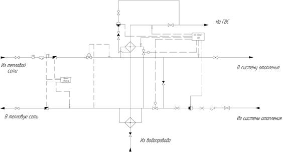
In the heat supply system, the heat point connecting the heat network with the heat consumer occupies an important place. By means of a heat point (TP), local consumption systems (heating, hot water supply, ventilation) are controlled, it also transforms the coolant parameters (temperature, pressure, maintaining a constant flow rate, heat accounting, etc.). At the same time, the network itself is controlled in the heating point, since it distributes the coolant in relation to the heating network and controls its parameters.
We carry out the project of a heating point for a 5-storey building connected on site 6.
The scheme of an individual heat point is given
Selection of mixing pumps
The pump flow is determined in accordance with SP 41-101-95 by the formula:
where is the estimated maximum water consumption for heating from the heating network kg / s;
u- mixing coefficient, determined by the formula:
where is the temperature of the water in the supply pipeline of the heating network at the design outdoor temperature for heating design t n.o, °С;
- also, in the supply pipeline of the heating system, ° С;
- the same, in the return pipeline from the heating system, °С;
![]() ;
;
The pressure of the mixing pump with such installation schemes is determined depending on the pressure in the heating network, as well as the required pressure in the heating system, and is taken with a margin of 2-3 m.
We choose circulation pumps WiloStratos ECO 30/1-5-BMS. These are standard pumps with a wet rotor and flange connection. The pumps are designed for use in heating systems, industrial circulation systems, water supply and air conditioning systems.
WiloStratos ECO are successfully used in systems where the temperature of the pumped liquid is in a wide range: from -20 to +130°C. A multi-stage (2, 3) speed switch allows the equipment to adapt to the current conditions of the heating system.
We install 2 Wilo pumps of the ECO 30/1-5-BMS brand with a flow of 3 m ^ 3 / h, a head of 6 m. One of the pumps is in reserve.
Selection circulation pump
We select a circulation pump of the GrundfosComfort type. These pumps circulate the water in the DHW system. Thanks to this, hot water flows immediately after the tap is opened. This pump is equipped with a built-in thermostat that automatically maintains the set water temperature in the range from 35 to 65 °C. This is a wet rotor pump, but due to its spherical shape, it is practically impossible to block the impeller due to contamination of the pump by impurities contained in the water. We choose a Grundfos UP 15-14 B pump with a flow rate of 0.8 m 3 / hour, a head of 1.2 m, and a power of 25 watts.
Selection of Magnetic Flanged Filters
Magnetic filters are designed to capture persistent mechanical impurities (including ferromagnets) in non-aggressive liquids with temperatures up to 150 ° C and a pressure of 1.6 MPa (16 kgf / cm 2). They are installed in front of cold and hot water. We accept the FMF filter.
The choice of sump
Mud collectors are designed to purify water in heat supply systems from suspended particles of dirt, sand and other impurities.
We install a sump series Du65 Ru25 T34.01 p.4.903-10 on the supply pipeline when entering the heating point.
Selecting a flow and pressure regulator
The regulator is used as a direct action regulator for automation of subscriber inputs of residential buildings. It is selected according to the coefficient bandwidth valves:
where D R= 0.03 ... 0.05 MPa - pressure drop across the valve, we accept D R= 0.04 MPa.
![]() m 3 / h.
m 3 / h.
The choice of flow and pressure regulator Danfoss AVP with a nominal diameter, D y - 65 mm, - 2 m 3 / h
Choosing a thermostat
Designed for automatic temperature control in open systems DHW. The regulator is equipped with a blocking device that protects the heating system from emptying during DHW peak hours and in emergency situations.
We choose a DanfossAVT / VG thermostat with a nominal diameter, D y - 65 mm, - 2 m 3 / h.
Check valve selection
Check valves are shutoff valves. They prevent backflow of water.
Check valves type 402 from Danfoss are installed on the pipeline after the PP, on the jumper after the pumps, after the circulation pump, on the DHW pipeline.
Relief valve selection
Safety valves are a type of pipeline fittings designed to automatically protect the technological system and pipelines from an unacceptable increase in pressure of the working medium by partially dumping it from the protected system. The most common spring safety valves, in which the pressure of the working medium is counteracted by the force of a compressed spring. The direction of supply of the working medium is under the spool. The safety valve is most often connected to the pipeline using a flange, with the cap up.
We choose a safety spring valve without manual undermining 17nzh21nzh (SPPK4) with D y = 65 mm.
Selection of ball valves
On the supply pipeline from the heating network, as well as on the return, on the pipelines to the thermostat and after it, we install Ball Valves, carbon steel (stainless steel ball), welded, with handle, flanged, ( R y = 2.5 MPa) Jip type, Danfoss, s D y = 65 mm. On the circulation pipeline of the DHW line before and after the circulation pump, we install ball valves with D y = 65 mm. Before the flow line of the heating system and after the return line, ball valves with D y = 65 mm and s D y = 65 mm. On the jumper of the mixing pumps we install ball valves with D y = 65 mm.
Selecting a heat meter
Heat meters for closed heat supply systems are designed to measure the total amount of thermal energy and the total volumetric amount of heat carrier. We install the heat calculator Logic 9943-U4 with SONO 2500 CT flowmeter; Dy = 32 mm.
The heat meter is designed for operation in open and closed systems water heat supply from 0 to 175 ºС and pressure up to 1.6 MPa. The difference in water temperatures in the supply and return pipelines of the system is from 2 to 175 ºС. The device provides connection of two similar platinum resistance thermocouples and one or two flowmeters. Provides registration of indications of parameters in electronic archive. The device generates monthly and daily reports, where all the necessary information about the consumption of thermal energy and coolant is presented in tabular form.
A set of thermocouples KTPTR-01-1-80 platinum is designed to measure the temperature difference in the supply and return pipelines of heat supply systems. It is used as part of heat meters. The principle of operation of the set is based on the proportional change in the electrical resistance of two thermal converters matched in terms of resistance and temperature coefficient depending on the measured temperature. Temperature measurement range from 0 to 180 о С.
 Conclusion
The aim of the work was to develop a heating system for a residential microdistrict. The area consists of thirteen buildings, eleven residential, one Kindergarten and one school., the location of the district of Omsk.
The developed heat supply system is closed with central quality control with temperature chart 130/70. By the nature of the heat supply, it is two-stage - the buildings are directly connected to the heating network through automated ITPs, there are no central heating stations.
When developing the heating network, the following necessary calculations were performed:
Definitely thermal loads for heating, ventilation and hot water supply of all subscribers. As a method for determining the loads of heating and ventilation, the method of aggregated indicators was used. Based on the type and volume of the building, specific heat losses of the building were set. Design temperatures are taken according to the outside temperature according to SNiP "Construction Climatology". Indoor temperature according to reference data according to SanPiN based on the purpose of the room. The load on hot water supply was determined by the standard consumption of hot water per person according to reference data based on the type of building.
The schedule of the central quality regulation is calculated
Definitely settlement costs network water (subscribers)
A hydraulic diagram of the heating network has been developed and a hydraulic calculation has been performed, the purpose of which is to determine the diameters of pipelines and the pressure drop in sections of the heating network
The thermal calculation of heat pipelines has been performed, i.e. calculation of insulation to reduce heat loss in the network. The calculation was made according to the method of not exceeding the normalized heat losses. A pre-insulated pipe with polyurethane foam insulation was chosen as the heat conductors. Pipeline laying method channelless
Compensators were selected to compensate for elongation of pipelines due to thermal expansion. Bellows expansion joints are used as compensators.
 - a scheme of an individual heating point was developed and the main elements were selected, i.e. pumps, control valves, thermostats, etc.
Bibliographic list
1. Sokolov E.Ya. Heating and heating networks / E.Ya.Sokolov; .– M.: MPEI Publishing House, 2001. – 472 p.: ill.
2. Tikhomirov A.K. Heat supply of the city district: textbook. Allowance / A.K. Tikhomirov.- Khabarovsk: Tkhookean Publishing House. State. University, 2006.-135p.
3. Manyuk V.I. Adjustment and operation of water heating networks: a Handbook./ V.I. Manyuk, E.B. Khizh and others. M.: Stroyizdat, 1988. 432s.
4. Designer's Handbook. Designing of thermal networks./Ed. A.A. Nikolaev. M. 1965. 359s.
5. Zinger N.M. Hydraulic and thermal regimes of heating systems. M.: Energoatomizdat, 1986. 320s.
6. Zlatopolsky A.N. Economics, organization and planning of thermal power facilities industrial enterprise/ Zlatopolsky A.N., Pruzner S.L., Kalinina E.I., Voroshilov B.S. M.: Energoatomizdat, 1995. 320s.
7. Collection No. 24 "Heat supply and gas pipelines - external networks" TER 81-02-24-2001 (Omsk), 2002.
8. SNiP 41-03-2003 Thermal insulation.
9. I.V. Belyaykina Water heating networks / I.V. Belyaikina, V.P. Vitaliev, N.K. Gromov and others; Ed. N.K. Gromova, E.P. Shubin. Moscow: Energoatomizdat, 1988 376s.
10. SNiP 41-02-2003 Heating networks.
11. Kozin V.E. Heat supply / Kozin V.E., Levina T.A., Markov A.P., Pronina I.B., Slemzin V.A. M.: graduate School, 1980. 408s.
12.Heat supply ( course design): Textbook / V. M. Kopko, N.K. Zaitsev, G. I. Bazylenko-Mn, 1985-139 p.
13. SNiP 23-01-99* "Construction climatology"
14 Application of Danfoss Automation Tools in Heating Points of Building District Heating Systems, V.V. Nevsky, 2005
15. Danfoss standard automated block heat points, V.V. Nevsky, D.A. Vasiliev, 2008
16 Design of district heating distribution networks,
E.V. Korepanov, M.: Higher school, 2002,
Hello! The main purpose of hydraulic calculation at the design stage is to determine the diameters of pipelines for given coolant flow rates and available pressure drops in the network, or in separate sections of the heating network. During the operation of networks, one has to solve the inverse problem - to determine the flow rates of the coolant in sections of the network or the pressure at individual points when changing hydraulic regimes. Without calculations for hydraulics, it is impossible to build a piezometric graph of the heating network. Also, this calculation is necessary to select the connection scheme internal system heat supply directly from the consumer and the choice of network and make-up pumps.
As you know, the hydraulic losses in the network are made up of two components: from the hydraulic linear friction losses and pressure losses in local resistances. By local resistances are meant - valves, turns, compensators, etc.
That is, ∆P = ∆Pl + ∆Pplace,
Linear friction losses are determined from the formula:
where λ is the coefficient hydraulic friction; l is the length of the pipeline, m; d is the internal diameter of the pipeline, m; ρ is the heat carrier density, kg/m³; w² is the speed of the coolant, m/s.
In this formula, the coefficient of hydraulic friction is determined by the formula of A.D. Altshul:
where Re is the Reynolds number, ke/d is the equivalent pipe roughness. These are reference values. Losses in local resistances are determined by the formula:
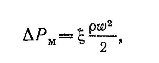
where ξ is the total coefficient of local resistances. It must be calculated manually using tables with local resistance coefficient values. In the Excel calculation attached to the article, I added a table with local resistance coefficients.
To perform a hydraulic calculation, you will definitely need a heat network diagram, something like this:
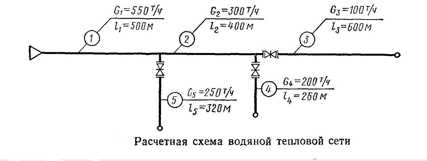
In fact, the scheme, of course, should be more detailed and detailed. I gave this diagram only as an example. From the heating network diagram, we need such data as: the length l of the pipeline, the flow rate G, and the diameter of the pipeline d.
How to perform a hydraulic calculation? The entire heating network that needs to be calculated is divided into so-called settlement sections. The calculated section is a section of the network where the flow rate does not change. First, hydraulic calculation is carried out in sections in the direction of the main line, which connects the heat source to the most remote heat consumer. Then, secondary directions and branches of the heating network are already calculated. My hydraulic calculation of the heating network section can be downloaded here:
This, of course, is the calculation of only one branch of the heating network (hydraulic calculation of a long-distance heating network is a rather laborious task), but it is enough to understand what the calculation of hydraulics is, and even for an unprepared person to start calculating hydraulics.
I will be glad to comments on the article.